The Structure of Neuron
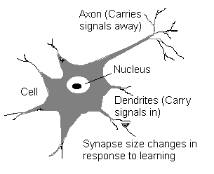
Source of the diagram: NIBS Pte Ltd.
|
Neural Doctrine |
The nervous system of living organisms is a structure consisting of many elements working in parallel and in connection with one another |
|
1836 |
Discovery of the neural cell of the brain, the neuron |
|
The Structure of Neuron |
Source of the diagram: NIBS Pte Ltd. |
This is a result worth of the Nobel Prize [1906]. The neuron is a many-inputs / one-output unit. The output can be excited or not excited , just two possible choices (like a flip-flop). The signals from other neurons are summed together and compared against a threshold to determine if the neuron shall excite ("fire"). The input signals are subject to attenuation in the synapses which are junction parts of the neuron.
|
1897 |
Synapse concept introduced |
The next important step was to find that the synapse resistance to the
incoming signal can be changed during a "learning" process [1949]:
|
Hebb's Learning Rule |
If an input of a neuron is repeatedly and persistently causing the neuron to fire, a metabolic change happens in the synapse of that particular input to reduce its resistance. |
This discovery became a basis for the concept of associative memory (see below).
|
1943 |
First mathematical representation of neuron |
|
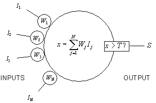
Artificial Neuron |
|
The Artificial Neuron is actually quite simple. All signals can be 1 or -1 (the "binary" case, often called classic spin for its similarity with the problem of disordered magnetic systems). The neuron calculates a weighted sum of inputs and compares it to a threshold. If the sum is higher than the threshold, the output is set to 1, otherwise to -1.
The power of neuron comes from its collective behavior in a network where all neurons are interconnected. The network starts evolving: neurons continuously evaluate their output by looking at their inputs, calculating the weighted sum and comparing to a threshold to decide if they should fire. This is highly complex parallel process whose features can not be reduced to phenomena taking place with individual neurons.
One observation is that the evolving of ANN causes it to eventually reach a state where all neurons continue working but no further changes in their state happen. A network may have more than one stable states, and it is obviously determined (somehow) by the choice of synaptic weights and thresholds for the neurons.
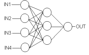
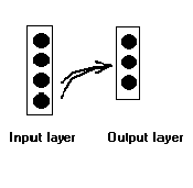
Another step in understanding of ANN dynamics was made with introduction
and analysis of a perceptron [Rosenblat, 1958], a simple neural network consisting
of input layer, output layer, and possibly one or more intermediate layers
of neurons.
|
Perceptron |
|
Once the input layer neurons are clamped to their values, the evolving starts: layer by layer, the neurons determine their output. This ANN configuration is often called feed-forward because of this feature. The dependence of output values on input values is quite complex and includes all synaptic weights and thresholds. Usually this dependence does not have a meaningful analytic expression. However, this is not necessary: there are learning algorithms that, given the inputs, adjust the weights to produce the required output.
So, simply put, we created a thing which learns how to recognize certain input patterns.
There is a training phase when known patterns are presented to the network and its weights are adjusted to produce required outputs. Then, there is a recognition phase when the weights are fixed, the patterns are again presented to the network and it recalls the outputs.
Among many applications of the feed-forward ANNs, the classification
or prediction scenario is perhaps the most interesting for data mining.
In this mode, the network is trained to classify certain patterns into certain
groups, and then is used to classify novel patterns which were never
presented to the net before. (The correct term for this scenario is schemata-completion
).
|
Example (courtesy Trajecta ) |
A company plans to suggest a product to potential customers. A database of 1 million customer records exists; 20,000 purchases (2% response) is the goal. Instead of contacting all 1,000,000 customers, only 100,000 is contacted. The response to the sale offers is known; so the subset is used to train a neural network to tell which of the 100,000 customers decide to buy the product. Then the rest 900,000 customers are presented to the network which classifies 32,000 of them as buyers. The 32,000 customers are contacted. and the 2% response is achieved. Total savings $2,500,000. |
The most popular algorithm for adjusting weights during the training phase is called back-propagation of error. The initial configuration of ANN is arbitrary; the result of presenting a pattern to the ANN is likely to produce incorrect output. The errors for all input patterns are propagated backwards, from the output layer towards the input layer. The corrections to the weights are selected to minimize the residual error between actual and desired outputs. The algorithm can be viewed as a generalized least squares technique applied to multilayer perceptron. The usual approach of minimizing the errors leads to a system of linear equations; it is important to realize here that its solution is not unique. The time spent on calculating weights is much longer than the time required to run the finalized neural network in the recognition mode, so the resulting weights are arguably eligible for copyright protection.
Introduction of an energy function concept, due to Hopfield [1982-1986],
led to an explosion of work on neural networks. The energy function brought
an elegant answer to a tough problem of ANN convergence to a stable state:
|
Energy Function |
(A network of N neurons with weights Wij and output states Si ) |
The specifics of ANN evolving allowed to introduce this function which always
decreases (or remains unchanged) with each iteration step. Evolving of ANNs
and even their specifications started to be described in terms of the energy
function.
Apparently, letting an ANN to evolve eventually shall lead it to a stable
state where the energy function has a minimum and can not change further.
The information stored in the synaptic weights Wij therefore
corresponds to some minima of the energy function where the neural network
ends up after its evolving.
|
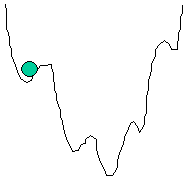
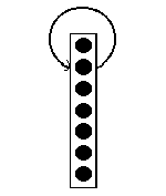
Minima of Energy Function |
|
When the input neurons are clamped to the initial values, the network obtains certain energy as indicated by a ball in the above figure. Further evolving will cause the ball to slide to the nearest local minimum.
Training of a network is adjustment of weights to match the actual outputs to desired outputs of the network. The expression for the energy function contain the weights, and we can think of the training process as "shaping" of the energy function.
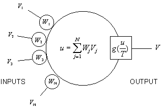
The Mean Field Theory (MFT) [Hopfield, 1982] treats neurons as objects with continuous inputs and output states, not just +1 or -1, as in the "classic spin" approach. In the network of neurons, MFT introduces statistical notion of "thermal average", "mean" field V of all input signals of a neuron. To provide the continuity of the neuron outputs, a notion of sigmoid function, g(u), is introduced to be used instead of a simple step-function threshold.
|
Classic Spin |
Mean Field |
|
| Neuron State | Si = -1 or +1 | |
| Energy | ||
| Neuron Input Field | ||
| Evolving | Si = sign( Ui ) |
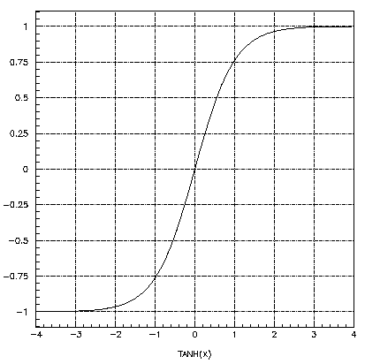
The most popular sigmoid function for ANNs is tanh:
|
Sigmoid Function |
|
Sigmoid function makes processing in neurons nonlinear:
|
Artificial Neuron, MFT |
|
This configuration of neural networks does not assume propagation of input signal through the hidden layers to the output layers; rather, the output signals of neurons are fed again to the inputs so that evolving continues until stopped externally
|
Feed-forward |
Feed-back |
|
|
|
The feed-back ANNs best suited for optimization problems where the neural network looks for the best arrangement of interconnected factors. The arrangement corresponds to the global minimum of the energy function (see section 3.2.2). Feed-back ANNs are also used for error-correction and partial-contents memories (see section 3.1.3) where the stored patterns correspond to the local minima of the energy function.
Optimization problems require a search for the global minimum of the energy function. If we simply let ANN evolve it will reach the nearest local minimum and stop there. To help with the search, one way is to allow for energy fluctuations in ANN by introducing a "probability" that the neuron should fire when the local field is high or should stay calm if the local field is low. In other words, certain amount of chaos is introduced into the ANN evolving process, which can be also imagined as "shaking" of the system where the ball slides along the energy function curve.
If we allow "shaking" of the evolving process, it is important not to shake the system out of the global minimum. In other words, shaking should be made lighter as the network evolves. Due to similarity of annealing technique used in metal industry, the temperature scenarios are collectively called simulated annealing. There are a few popular stochastic simulated annealing schemes (Heat Bath, Metropolis, Langevin).
Training of the neural networks is an optimization problem itself. Simulated annealing schemes are applied there, too (see Section 4.2).
Treatment of ANN evolving within the MFT approach allows for tunneling of the energy into the neighboring (lower) maximum of the energy function.
4.1.1. Fitting the Data
Application of neural networks to Data Mining uses the ability of ANN to build models of data by capturing the most important features during training period. What is called "statistical inference" in statistics, here is called "data fitting". The critical issue in developing a neural network is this generalization: how well will the network make classification of patterns that are not in the training set? Neural networks, like other flexible nonlinear estimation methods such as kernel regression and smoothing splines, can suffer from either underfitting or overfitting.
The training set of data might as well be quite "noisy" or "imprecise". The training process usually relies on some version of least squares technique which ideally should abstract from the noise in the data. However, this feature of ANN is dependent on how optimal is the configuration of the net in terms of number of layers, neurons and, ultimately, weights.
|
Underfitting |
ANN that is not sufficiently complex to correctly detect the pattern in a noisy data set. |
|
Overfitting |
ANN that is too complex so it reacts on noise in the data |
A network that is not sufficiently complex can fail to detect fully the
signal in a complicated data set, leading to underfitting. A network that
is too complex may fit the noise, not just the signal, leading to overfitting.
Overfitting is especially dangerous because it can easily lead to predictions
that are far beyond the range of the training data with many of the common
types of neural networks. But underfitting can also produce wild predictions
in multilayer perceptrons, even with noise-free data.
4.1.3. Avoiding Underfitting and Overfitting
The best way to avoid overfitting is to use lots of training data. If
you have at least 30 times as many training cases as there are weights in
the network, you are unlikely to suffer from overfitting. But you can't arbitrarily
reduce the number of weights for fear of underfitting.
Given a fixed amount of training data, there are at least five effective
approaches to avoiding underfitting and overfitting, and hence getting good
generalization:
Training a neural network is, in most cases, an exercise in numerical optimization of a usually nonlinear function. Methods of nonlinear optimization have been studied for hundreds of years, and there is a huge literature on the subject in fields such as numerical analysis, operations research, and statistical computing, e.g., Bertsekas 1995, Gill, Murray, and Wright 1981. There is no single best method for nonlinear optimization. You need to choose a method based on the characteristics of the problem to be solved. For functions with continuous second derivatives (which would include feedforward nets with the most popular differentiable activation functions and error functions), three general types of algorithms have been found to be effective for most practical purposes: For a small number of weights, stabilized Newton and Gauss-Newton algorithms, including various Levenberg-Marquardt and trust-region algorithms are efficient. For a moderate number of weights, various quasi-Newton algorithms are efficient. For a large number of weights, various conjugate-gradient algorithms are efficient. All of the above methods find local optima. For global optimization, there are a variety of approaches. You can simply run any of the local optimization methods from numerous random starting points. Or you can try more complicated methods designed for global optimization such as simulated annealing or genetic algorithms (see Reeves 1993 and "What about Genetic Algorithms and Evolutionary Computation?").