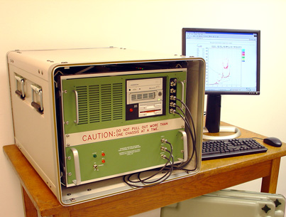
Figure 1-1A DigisondeTM Portable Sounder |
Figure
1-1B Magnetic Loop Turnstile Antenna |
Noteworthy
new technology involved in this system includes:
-
Electronically
switched active crossed loop receiving antenna
-
Commercially
sourced 10 MIPS TMS 320C25 digital signal processor
(DSP)
-
4
million sample DSP buffer memory
-
71
to 110 MHz digital synthesizer on a 4"x5"
card
-
Compact
DC-DC converters allowing operation on one battery
-
Four-channel
high speed (1 million 12-bit samples/sec) digitizer
board
-
A
160 Mbits/sec parallel data bus between the digitizer
and the DSP
-
A
proprietary multi-tasking operating system for remote
interaction via a modem connection without suspending
system operation
-
Direct
digital synthesized coherent oscillators
-
21
dB signal processing gain from phase coded pulse compression
-
21
dB additional signal processing gain from coherent
Doppler integration
-
Automatic
ionospheric layer identification and parameter scaling
by an embedded expert system
The
availability of a small low power ionosonde that could be
operated on-site wherever a high frequency (HF) radio or
radar was in use, would greatly increase the value of the
information produced by the instrument since it would become
available to the end user immediately.
One
of the chief applications for the real-time data currently
provided by digital ionospheric sounders is to manage the
operation of HF radio channels and networks. Since many
HF radios are operated at remote locations (i.e., aircraft,
boats, land vehicles of all sorts, and remote sites where
telephone service is unreliable) the major obstacle to making
practical use of the ionospheric sounder data and associated
computed propagation information is the dissemination of
this data to a data processing and analysis site. Since
HF is often used where no alternative communications link
exists, or is held in reserve in case primary communication
is lost, it is not practical to assume that a communications
link exists to make centrally tabulated real-time ionospheric
data available to the user. Furthermore, local measurements
are superior to measurements at sites of opportunity in
the user’s general region of the globe since extreme
variations in ionospheric properties are possible even over
short distances, especially at high latitudes [Buchau et
al., 1985; Buchau and Reinisch, 1991] or near the sunset
or sunrise terminator.
However,
for most applications, the size, weight, power consumption
and cost of a conventional ionospheric sounder have made
local measurements impractical. Therefore the availability
of a small, low cost sounder is a major improvement in the
usefulness of ionospheric sounder data. Shrinking the conventional
1 to 50 kW pulse sounders to a portable, battery operated
100 to 500 W system requires the application of substantial
signal processing gain to compensate for the 20 dB reduction
in transmitter power. Furthermore, a compact portable package
requires the use of highly integrated control, data acquisition,
timing, data processing, display and storage hardware.
The
objective of the DPS development project was to develop
a small vertical incidence (i.e., monostatic) ionospheric
sounder which could automatically collect and analyze ionospheric
measurements at remote operating sites for the purpose of
selecting optimum operating frequencies for obliquely propagated
communication or radar propagation paths. Intermediate objectives
assumed to be necessary to produce such a capability were
the development of optimally efficient waveforms and of
functionally dense signal generation, processing and ancillary
circuitry. Since the need for an embedded general purpose
computer was a given imperative, real-time control software
was developed to incorporate as many functions as was feasible
into this computer rather than having to provide additional
circuitry and components to perform these functions. The
DPS duplicates all of the functions of its predecessor the
DigisondeTM 256 [Bibl et al., 1981] and [Reinisch,
1987] in a much smaller, low power package. These include
the simultaneous measurement of seven observable parameters
of reflected (or in oblique incidence, refracted) signals
received from the ionosphere:
1)
Frequency
2) Range (or height for vertical incidence measurements)
3) Amplitude
4) Phase
5) Doppler Shift and Spread
6) Angle of Arrival
7) Wave Polarization
Because
the physical parameters of the ionospheric plasma affect
the way radio waves reflect from or pass through the ionosphere,
it is possible by measuring all of these observable parameters
at a number of discrete heights and discrete frequencies
to map out and characterize the structure of the plasma
in the ionosphere. Both the height and frequency dimensions
of this measurement require hundreds of individual measurements
to approximate the underlying continuous functions. The
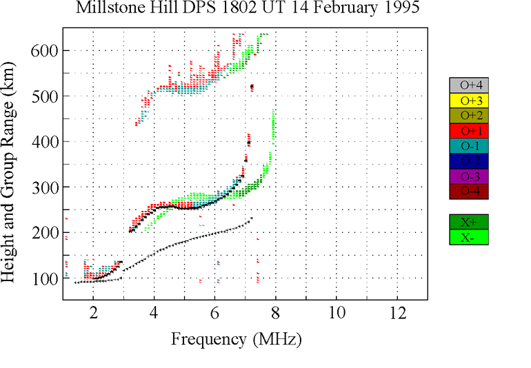
resulting measurement is called an ionogram and comprises
a seven dimensional measurement of signal amplitude vs.
frequency and vs. height as shown in Figure 1-2 (due to
the limitations of current software only five may be displayed
at a time). Figure 1-2 is a five-dimensional display, with
sounding frequency as the abscissa, virtual reflection height
(simple conversion of time delay to range assuming propagation
at 3x10⁸ m/sec) as the ordinate, signal amplitude
as the spot (or pixel) intensity, Doppler shift as the color
shade and wave polarization as the color group (the blue-green-grey
scale or "cool" colors showing extraordinary polarization,
the red-yellow-white scale or "hot" colors showing
ordinary polarization).
Figure
1-2 Five-Dimensional Ionogram
Another
objective of the DPS development was to store the data created
by the system in an easily accessible format (e.g., DOS
formatted personal computer files), while maintaining compatibility
with the existing base of DigisondeTM sounder
analysis software in use at the UMLCAR and at over 40 research
institutes around the world. This objective often competed
with the additional objective of providing an easily accessible
and simply understood standard data format to facilitate
the development of novel post-processing analysis and display
programs.
Ionospheric
Propagation of Electromagnetic Waves back
to top
An
ionospheric sounder uses basic radar techniques to detect
the electron density (equal to the ion density since the
bulk plasma is neutral) of ionospheric plasma as a function
of height. The ionospheric plasma is created by energy from
the sun transferred by particles in the solar wind as well
as direct radiation (especially ultra-violet and x-rays).
Each component of the solar emissions tends to be deposited
at a particular altitude or range of altitudes and therefore
creates a horizontally stratified medium where each layer
has a peak density and to some degree, a definable width,
or profile. The shape of the ionized layer is often referred
to as a Chapman function [Davies, 1989] which is a roughly
parabolic shape somewhat elongated on the top side. The
peaks of these layers usually form between 70 and 300 km
altitude and are identified by the letters D, E, F1 and
F2, in order of their altitude.
By
scanning the transmitted frequency from 1 MHz to as high
as 40 MHz and measuring the time delay of any echoes (i.e.,
apparent or virtual height of the reflecting medium) a vertically
transmitting sounder can provide a profile of electron density
vs. height. This is possible because the relative refractive
index of the ionospheric plasma is dependent on the density
of the free electrons (Ne), as shown in Equation
1-1 (neglecting the geomagnetic field):
m2(h)= 1 – k (Ne/f2)
(1–1)
where k
= 80.5, Ne is electrons/m3, and f
is in Hz [Davies, 1989; Chen, 1987].
The
behavior of the plasma changes significantly in the presence
of the Earth’s magnetic field. An exhaustive derivation
of m [Davies, 1989] results in the Appleton Equation for
the refractive index, which is one of the fundamental equations
used in the field of ionospheric propagation. This equation
clearly shows that there are two values for refractive index,
resulting in the splitting of a linearly polarized wave
incident upon the ionosphere, into two components, known
as the ordinary and extraordinary waves. These propagate
with a different wave velocity and therefore appear as two
distinct echoes. They also exhibit two distinct polarizations,
approximately right hand circular and left hand circular,
which aid in distinguishing the two waves.
When
the transmitted frequency is sufficient to drive the plasma
at its resonant frequency there is a total internal reflection.
The plasma resonance frequency (fp) is defined
by several constants, e – the charge of an electron,
m – the mass of an electron, eo
– the permittivity of free space, but only one variable,
Ne – electron density in electrons/m3
[Chen, 1987]:
fp2 = (Ne e2/4peom) = kNe (1-2)
A
typical number for the F-region (200 to 400 km altitude)
is 1012 electrons/m3, so the plasma
resonance frequency would be 9 MHz. The value of m
in Equation 1–1 approaches 0 as the operating frequency,
f, approaches the plasma frequency. The group velocity of
a propagating wave is proportional to m,
so
m
= 0 implies that the wave slows down to zero which is obviously
required at some point in the process of reflection since
the propagation velocity reverses.
The
total internal reflection from the ionosphere is similar
to reflection of radio frequency (RF) energy from a metal
surface in that the re-radiation of the incident energy
is caused by the free electrons in the medium. In both cases
the wave penetrates to some depth. In a plasma the skin
depth (the depth into the medium at which the electric field
is 36.8% of its incident amplitude) is defined by:
          l0/2p
    d =  ----------			                (1-3)

where l0 is
the free space wavelength.
The
major difference between ionospheric reflection and reflection
from a metallic surface is that the latter has a uniform
electron density while the ionospheric density increases
roughly parabolically with altitude, with densities starting
at essentially zero at stratospheric altitudes and rising
to a peak at about 200 to 400 km. In the case of a metal
there is no region where the wave propagates below the resonance
frequency, while in the ionosphere the refractive index
and therefore the wave velocity change with altitude until
the plasma resonance frequency is reached. Of course if
the RF frequency is above the maximum plasma resonance frequency
the wave is never reflected and can penetrate the ionosphere
and propagate into outer space. Otherwise what happens on
a microscopic scale at the surface of a metal and on a macroscopic
scale at the plasma resonance in the ionosphere is very
similar in that energy is re-radiated by electrons which
are responding to the incident electric field.
Coherent Integration
back to top
During
the 1960’s and 1970’s several variations in sounding
techniques started moving significantly beyond the basic
pulse techniques developed in the 1930’s. First was
the coherent integration of several pulses transmitted at
the same frequency. Two signals are coherent if, having
a phase and amplitude, they are able to be added together
(e.g., one radar pulse echo received from a target added
to the next pulse echo received from the same target, thousandths
of a second later) in such a way that the sum may be zero
(if the two signals are exactly out of phase with each other)
or double the amplitude (if they are exactly in phase).
Coherent integration of N signals can provide a factor of
N improvement in power. This technique was first used in
the DigisondeTM 128 [Bibl and Reinisch, 1975].
In
ionospheric sounding, the motion of the ionosphere often
makes it impossible to integrate by simple coherent summation
for longer that a fraction of a second, although it is not
rare to receive coherent echoes for tens of seconds. However,
with the application of spectral integration (which is a
byproduct of the Fourier transform used to create a Doppler
spectrum) it is possible to coherently integrate pulse echoes
for tens of seconds under nearly all ionospheric conditions
[Bibl and Reinisch, 1978]. The integration may progress
for as long a time as the rate of change of phase
remains constant (i.e., there is a constant Doppler shift,
Df).
The DigisondeTM 128PS, and all subsequent versions
perform this spectral integration.
Additional
detail on this topic is contained in Chapter 2 in this section.
Coded Pulses
to Facilitate Pulse Compression Radar Techniques back
to top
A
third general technique to improve on the simple pulse sounder
is to stretch out the pulse by a factor of N, thus increasing
the duty cycle so the pulse contains more energy without
requiring a higher power transmitter (power x time = energy).
However, to maintain the higher range resolution of the
simple short pulse the pulse can be bi-phase, or phase reversal
modulated with a phase code to enable the receiver to create
a synthetic pulse with the original (i.e., that of the short
pulse) range resolution. A network of sounders using a 13-bit
Barker Code were operated by the U.S. Navy in the 1960’s.
The
critical factor in the use of pulse compression waveforms
for any radar type measurement is the correlation properties
of the internal phase code. Phase codes proposed and experimented
with included the Barker Code [Barker, 1953], Huffman Sequences
[Huffman 1962], Convoluted Codes [Coll, 1961], Maximal Length
Sequence Shift Register Codes (M-codes) [Sarwate and Pursley,
1980], or Golay’s Complementary Sequences [Golay, 1961],
which have been implemented in the VHF mesospheric sounding
radar at Ohio State University [Schmidt et al., 1979] and
in the DPS. The internal phase code alternative has just
recently become economically feasible with the availability
of very fast microprocessor and signal processor IC’s.
Barker Coded pulses have been implemented in several ionospheric
sounders to date, but until the DPS was developed there
have been no other successful implementations of Complementary
Series phase codes in ionospheric sounders.
The
European Incoherent Scatter radar in Tromso, Norway (VanEiken,
1991 and 1993) and an over-the-horizon (OTH) HF radar used
the Complementary Series codes. However most major radar
systems including all currently active OTH radars opted
for the FM/CW chirp technique, due to its resistance to
Doppler induced leakage and its compatibility with analog
pulse compression processing techniques. Basically, the
chirp waveform avoids the need for extremely fast digital
processing capabilities, since only the final stage is performed
digitally, while the pulse compression is best performed
entirely digitally. Even at the modest bandwidths used for
ionospheric sounding, this digital capability was until
recently, much more expensive and cumbersome than the special
synthesizers required for chirpsounding.
Another
new development in the 1970’s was the coherent multiple
receiver array [Bibl and Reinisch, 1978] which allows angle
of arrival (incidence angle) to be deduced from phase differences
between antennas by standard interferometer techniques.
Given a known operating frequency, and known antenna spacing,
by measuring the phase or phase difference on a number of
antennas, the angle of arrival of a plane wave can be deduced.
This interferometry solution is invalid, however, if there
are multiple sources contributing to the received signal
(i.e., the received wave therefore does not have a planar
phase front). This problem can be overcome in over 90% of
the cases as was first shown with the DigisondeTM
256 [Reinisch et al., 1987] by first isolating or discriminating
the multiple sources in range, then in the Doppler domain
(i.e., isolating a plane wavefront) before applying the
interferometry relationships.
Except
for the FM/CW chirpsounder which operates well on transmitter
power levels of 10 to 100 W (peak power) the above techniques
and cited references typically employ a 2 to 30 kW peak
power pulse transmitter. This power is needed to get sufficient
signal strength to overcome an atmospheric noise environment
which is typically 20 to 50 dB (CCIR Noise Tables) above
thermal noise (defined as kTB, the theoretical minimum noise
due to thermal motion, where k = Boltzman’s constant,
T = temperature in °
K, and
B = system bandwidth in Hz). More importantly, however,
since ionogram measurements require scanning of the entire
propagating band of frequencies in the 0.5 to 20 MHz RF
band (up to 45 MHz for oblique measurements), the sounder
receiver will encounter broadcast stations, ground-to-air
communications channels, HF radars, ship-to-shore radio
channels and several very active radio amateur bands which
can add as much as 60 dB more background interference. Therefore,
the sounder signal must be strong enough to be detectable
in the presence of these large interfering signals.
To
make matters worse, a pulse sounder signal must have a broad
bandwidth to provide the capability to accurately measure
the reflection height, therefore the receiver must have
a wide bandwidth, which means more unwanted noise is received
along with the signal. The noise is distributed quite evenly
over bandwidth (i.e., white), while interfering signals
occur almost randomly (except for predictably larger probabilities
in the broadcast bands and amateur radio bands) over the
bandwidth. Thus a wider-bandwidth receiver receives proportionally
more uniformly distributed noise and the probability of
receiving a strong interfering signal also goes up proportionally
with increased bandwidth.
The
DPS transmits only 300 W of pulsed RF power but compensates
for this low power by digital pulse compression and coherent
spectral (Doppler) integration. The two techniques together
provide about 30 dB of signal processing gain (up to 42
dB for the bi-static oblique waveforms) thus for vertical
incidence measurements the system performs equivalently
with a simple pulse sounder of 1000 times greater power
(i.e., 300 kW).
Additional
detail on this topic is contained in Chapter 2 in this section.
Current Applications
of Ionospheric Sounding back to top
Current
applications of ionospheric sounders fall into two categories:
a.
Support of operational systems, including shortwave radio
communications and OTH radar systems. This support can
be in the form of predictions of propagating frequencies
at given times and locations in the future (e.g., over
the ensuing month) or the provision of real-time updates
(updated as frequently as every 15 minutes) to detect
current conditions such that system operating parameters
can be optimized.
b.
Scientific research to enable better prediction of ionospheric
conditions and to understand the plasma physics of the
solar-terrestrial interaction of the Earth’s atmosphere
and magnetic field with the solar wind.
There
has been considerable effort in producing global models
of ionospheric densities, temperature, chemical constitution,
etc, such that a few sounder measurements could calibrate
the models and improve the reliability of global predictions.
It has been shown that if measurements are made within a
few hundred kilometers of each other, the correlation of
the measured parameters is very high [Rush, 1978]. Therefore
a network of sounders spaced by less than 500 km can provide
reliable estimates of the ionosphere over a 250 km radius
around them.
The
areas of research pursued by users of the more sophisticated
features of the DigisondeTM sounders include
polar cap plasma drift, auroral phenomena, equatorial spread-F
and plasma irregularity phenomena, and sporadic E-layer
composition [Buchau et al., 1985; Reinisch 1987; and Buchau
and Reinisch 1991]. There may be some driving technological
needs (e.g., commercial or military uses) in some of these
efforts, but many are simply basic research efforts aimed
at better understanding the manifestations of plasma physics
provided by nature.
Requirements
for a Small Flexible Sounding System back to
top
The detailed
design and synthesis of a RF measurement system (or any
electronic system) must be based on several criteria:
a. The
performance requirements necessary to provide the needed
functions, in this case scientific measurements of electron
densities and motions in the ionosphere.
b. The
availability of technology to implement such a capability.
c. The
cost of purchasing or developing such technology.
d. The
risk involved in depending on certain technologies, especially
if some of the technology needs to be developed.
e. The
capabilities of the intended user of the system, and its
expected willingness to learn to use and maintain it;
i.e., how complicated can the operation be before the
user will give up and not try to learn it.
The question
of what technology can be brought to bear on the realization
of a new ionospheric sounder was answered in a survey of
existing technology in 1989, when the portable sounder development
started in earnest. This survey showed the following available
components, which showed promise in creating a smaller,
less costly, more powerful instrument. Many of these components
were not available when the last generation of DigisondesTM
(circa 1980) was being developed:
Solid-state
300 W MOSFET RF power transistors
High-speed
high precision (12, 14 and 16 bit) analog to digital
(A–D) converters
High-speed
high precision (12 and 16 bit) digital to analog (D–A)
converters
Single
chip Direct Digital Synthesizers (DDS)
Wideband
(up to 200 MHz) solid state op amps for linear feedback
amplifiers
Wideband
(4 octaves, 2–32 MHz) 90°
phase shifters
Proven
DigisondeTM 256 measurement techniques
Very
fast programmable DSP (RISC) IC’s
Fast,
single board, microcomputer systems and supporting programming
languages
Many
of these components are inexpensive and well developed because
they feed a mass market industry. The MOSFET transistors are
used in Nuclear Magnetic Resonance medical imaging systems to
provide the RF power to excite the resonances. The high speed
D–A converters are used in high resolution graphic video
display systems such as those used for high performance workstations.
The DDS chips are used in cellular telephone technology, in
which the chip manufacturer, Qualcomm, is an industry leader.
The DSP chips are widely used in speech processing, voice recognition,
image processing (including medical instrumentation). And of
course, fast microcomputer boards are used by many small systems
integrators which end up in a huge array of end user applications
ranging from cash registers to scientific computing to industrial
process controllers.
The
performance parameters were well known at the beginning of the
DPS development, since several models of ionospheric pulse sounders
had preceded it. The frequency range of 1 to 20 MHz for vertical
sounding was an accepted standard, and 2 to 30 MHz was accepted
as a reasonable range for oblique incidence measurements. It
was well known that radio waves of greater than 30 MHz often
do propagate via skywave paths, however, most systems relying
on skywave propagation don’t support these frequencies,
so interest in this frequency band would only be limited to
scientific investigations. A required power level in the 5 to
10 kW range for pulse transmitters had provided good results
in the past. The measurement objectives were to simultaneously
measure all seven observable parameters outlined at Paragraph
107 above in order to characterize the following physical features:
The height
profile of electron density vs. altitude
Position
and spatial extent of irregularity structures, gradients and
waves
Motion vectors
of structures and waves
As
mentioned in the section above dealing with Current Applications
of Ionospheric Sounding (Paragraph 127 et seq. above),
the accurate measurement of all of the parameters, except frequency
(it being precisely set by the system and need not be measured)
depends heavily on the signal to noise ratio of the received
signal. Therefore vertical incidence ionospheric sounders capable
of acquiring high quality scientific data have historically
utilized powerful pulse transmitters in the 2 to 30 kW range.
The necessity for an extremely good signal to noise ratio is
demanded by the sensitivity of the phase measurements to the
random noise component added to the signal level. For instance,
to measure phase to 1 degree accuracy requires a signal to noise
ratio better than 40 dB (assuming a Gaussian noise distribution
which is actually a best case), and measurement of amplitude
to 10% accuracy requires over 20 dB signal to noise ratio. Of
course, is it desirable that these measurements be immune to
degradation from noise and interference and maintain their high
quality over a large frequency band. This requires that at the
lower end of the HF band the system’s design has to overcome
absorption, noise and interference, and poor antenna performance
and still provide at least a 20 to 40 dB signal to noise ratio.
METHODOLOGY,
THEORETICAL BASIS AND IMPLEMENTATION back to
top
General
The
VIS/DPS borrows several of the well proven measurement techniques
used by the DigisondeTM 256 sounder described in
[Bibl, et al, 1981; Reinisch et al., 1989] and [Reinisch, 1987],
which has been produced for the past 12 years by the UMLCAR.
The addition of digital pulse compression in the DPS makes the
use of low power feasible, the implementation in software of
processes that were previously implemented in hardware results
in a much smaller physical package, and the high level language
control software and standard PC-DOS (i.e., IBM/PC) data file
formats provide a new level of flexibility in system operation
and data processing.
A technical
description of the DPS (sounder unit and receive antennas sub-systems)
are contained in Section 2 of this manual.
Coherent
Phase Modulation and Pulse Compression back to
top
The
DPS is able to be miniaturized by lengthening the transmitted
pulse beyond the pulse width required to achieve the desired
range resolution where the radar range resolution is defined
as,
DR=c/2b       where b is the system bandwidth, or                                    (1-4)

DR=cT/2        for a simple rectangular pulse
                   waveform, with T being the width
                   of the rectangular pulse
The
longer pulse allows a small low voltage solid state amplifier
to transmit an amount of energy equal to that transmitted by
a high power pulse transmitter (energy = power x time, and power
= V2/R) without having to provide components to handle
the high voltages required for tens of kilowatt power levels.
The time resolution of the short pulse is provided by intrapulse
phase modulation using programmable phase codes (user selectable
and firmware expandable), the Complementary Codes, and M-codes
are standard. The use of a Complementary Code pulse compression
technique is described in this chapter, which shows that at
300 W of transmitter power the expected measurement quality
is the same as that of a conventional sounder of about 500 kW
peak pulse power.
The
transmitted spread spectrum signal s(t) is a biphase (180° phase
reversal) modulated pulse. As illustrated in Figure 1–3,
bi-phase modulation is a linear multiplication of the binary
spreading code p(t) (a.k.a. a chipping sequence, where each
code bit is a "chip") with a carrier signal sin(2pf0t) or in complex form,
exp[j2pf0t],
to create a transmitted signal,
s(t)=p(t)exp[j2pf0t] (1-5)
Figure 1-3 Generation of a Bi-phase Modulated Spread Spectrum Waveform
NOTE
Notation throughout this chapter
will use s(t) as the transmitted signal, r(t) the received
signal and p(t) as the chip sequence. Functions r1(t)
and r2(t) will be developed to describe
the signal after various stages of processing in the receiver.
The
term chip is used rather than bit because for
spread spectrum communications many chips are required to transmit
one bit of message information, so a distinct term had to be
developed. Figure 1-4 on the following page depicts the modulation
of a sinusoidal RF carrier signal by a binary code (notice that
the code is a zero mean signal, i.e., centred around 0 volts
amplitude). Since the mixer in Figure 1-3 can be thought of
as a mathematical multiplier, the code creates a 180o
(p radians)
phase shift in the sinusoidal carrier whenever p(t) is negative,
since –sin(wt) = sin(wt+p).
The
binary spreading code is identical to a stream of data bits
except that it is designed such that it forms a pattern with
uniquely desirable autocorrelation function characteristics
as described later in this chapter. The 16-bit Complementary
Code pair used in the DPS is 1-1-0-1-1-1-1-0-1-0-0-0-1-0-1-1
modulated onto the odd-numbered pulses and 1-1-0-1-1-1-1-0-0-1-1-1-0-1-0-0
modulated onto the even-numbered pulses. This pattern of phase
modulation chips is such that the frequency spectrum of such
a signal (as shown in Figure 1-4) is uniformly spread over the
signal bandwidth, thus the term "spread spectrum".
In fact, it is interesting to note that the frequency spectrum
content of the spread spectrum signal used by the DPS is identical
to that of the higher peak power, simple short pulse used by
the DigisondeTM 256, even though the physical pulse
is 8 times longer. Since they have the same bandwidth, Equation
1–4 would suggest that they have the same range resolution.
It will be shown later in this chapter, that the ability of
the DigisondeTM 256 and the DPS to determine range
(i.e., time delay), phase, Doppler shift and angle of arrival
is also identical between the two systems, even though the transmitted
waveforms appear to be vastly different.
Figure
1–4 Spectral Content of a Spread-Spectrum Waveform
Since
the transmitted signal would obscure the detection of the much
weaker echo in a monostatic system the transmitted pulse must
be turned off before the first E-region echoes arrive at the
receiver which, as shown in Figure 1-5, is about TE
= 600 m
sec after the beginning of the pulse. Also, since the receiver
is saturated when the transmitter pulse comes on again, the
pulse repetition frequency is limited by the longest time delay
(listening interval) of interest, which is at least 5 msec,
corresponding to reflections from 750 km altitude. To meet these
constraints, a 533 m
sec pulse made
up of eight 66.67 m sec phase
code chips (15 000 chips/sec) is selected which allows detection
of ionospheric echoes starting at 80 km altitude. To avoid excessive
range ambiguity, a highest pulse repetition frequency of 200
pps is chosen, which allows reception of the entire pulse from
a virtual height of 670 km (the pulse itself is 80 km long)
altitude before the next pulse is transmitted. This timing captures
all but the highest multihop F-region echoes which are of little
interest. Under conditions where higher unambiguous ranges,
and therefore longer receiver listening intervals, are desired
100 pps or 50 pps can be selected under software control.
Figure
1-5 Natural Timing Limitations for Monostatic Vertical Incidence
Sounding
The
key to the pulse compression technique lies in the selection
of a spreading function, p(t), which possesses an autocorrelation
function appropriate for the application. The ideal autocorrelation
function for any remote sensing application is a Dirac delta
function (or instantaneous impulse, d
(t) since this would provide perfect range accuracy and infinite
resolution. However, since the Dirac delta function has infinite
instantaneous power and infinite bandwidth, the engineering
tradeoffs in the design of any remote sensing system mainly
involve how far one can afford to deviate from this ideal (or
how much one can afford to spend in more closely approximating
this ideal) and still achieve the accuracy and resolution required.
More to the point, for a discussion of a discrete time digital
system such as the DPS, the ideal signal is a complex unit impulse
function, with the phase of the impulse conveying the RF phase
of the received signal. The many different pulse compression
codes all represent some compromise in achieving this ideal,
although each code has its own advantages, limitations, and
trade-offs. The autocorrelation function as applied to code
compression in the VIS/DPS is defined as:
       k
  R(k)=S p(n) p(n+k)                               (1-6)
       n
Therefore
the ideal as described above is R(k) = d(k).
(Several examples of autocorrelation functions of the codes
described in this Section can be seen in Figures 1-9 through
1-13.)
For
ionospheric applications, the received spread-spectrum coded
signal, r(t), may be a superposition of several multipath echoes
(i.e., echoes which have traveled over various propagation paths
between the transmitter and receiver) reflected at various ranges
from various irregular features in the ionosphere. The algorithm
used to perform the code compression operates on this received
multipath signal, r(t), which is an attenuated and time delayed
(possibly multiple time delays) replica of the transmitted signal
s(t) (from Equation 1–5), which can be represented as:
       P
  r(t)=S ai s(t-ti)    or                                    (1-7)
      i=1
       P
  r(t)=S ai  p(t-ti)exp[j2pf0t - fi]
      i=1
where
S
shows that the P multipath signals sum linearly at the receive
antenna, ai is the amplitude of the ith
multipath component of the signal, and ti
is the propagation delay associated with multipath i. The carrier
phase fi
of each multipath could be expressed in terms of the carrier
frequency and the time delay t
i
; however, since the multiple carriers (from the various multipath
components) cannot be resolved, while the delays in the complex
code modulation envelope can be, a separate term, f
i,
is used. Next, when the carrier is stripped off of the signal,
this RF phase term will be represented by a complex amplitude
coefficient ai
rather than ai.
Figure
1-6 Conversion to Baseband by Undersampling
By
down-converting to a baseband signal (a digital technique is
shown in Figure 1-6), the carrier signal can be stripped away,
leaving only the superposed code envelopes delayed by P multiple
propagation paths. Figure 1-6 presents one way to strip the
carrier off a phase modulated signal. This is the screen display
on a digital storage oscilloscope looking at the RF output from
the DPS system operating at 3.5 MHz. Notice that the horizontal
scan spans 2 msec, which if the oscilloscope was capable of
presenting more than 14 000 resolvable points, would display
7 000 cycles of RF. The sample clock in the digital storage
scope is not synchronized to the DPS, however, the digital sampling
remains coherent with the RF for periods of several milliseconds.
The analog signal is digitized at a rate such that each sample
is made an integer number of cycles apart (i.e., at the same
phase point) and therefore looks like a DC level until the phase
modulation creates a sudden shift in the sampled phase point.
Therefore the 180º phase reversals made on the RF carrier show
up as DC level shifts, replicating the original modulating code
exactly. The more hardware intensive method of quadrature demodulation
with hardware components (mixers, power splitters and phase
shifters) can be found in any communications systems textbook,
such as [Peebles, 1979]. After removing the carrier, the modified
r(t), now represented by r1(t) becomes:
      P
r1(t)=S ai p(t-ti)                                       (1-8)
     i=1
where
the carrier phase of each of the multipath components is now
represented by a complex amplitude a
i which carries along the RF phase term, originally defined
by f
i in Equation 1–7, for each multipath. Since
the pulse compression is a linear process and contributes no
phase shift, the real and imaginary (i.e., in-phase and quadrature)
components of this signal can be pulse compressed independently
by cross-correlating them with the known spreading code p(t).
The complex components can be processed separately because the
pulse compression (Equation 1–9B) is linear and the code
function, p(n), is all real. Therefore the phase of the cross-correlation
function will be the same as the phase of r1(t).
The
classical derivation of matched filter theory [e.g., Thomas,
1964] creates a matched filter by first reversing the time
axis of the function p(t) to create a matched filter impulse
response h(t) = p(–t). Implementing the pulse compression
as a linear system block (i.e., a "black box" with
impulse response h(t)) will again reverse the time axis of
the impulse response function by convolving h(t) with the
input signal. If neither reversal is performed (they effectively
cancel each other) the process may be considered to be a cross-correlation
of the received signal, r(t) with the known code function, p(t).
Either way, the received signal, r2(n) after matched
filter processing becomes:
r2(n)=r1(n)*h(n)=r1(n)*p(-n) (1-9A)
or by substituting
Equation 1–8 and writing out the discrete convolution,
we obtain the cross-correlation approach,
       P      M                         P
r2(n)=S ai  S p(k-ti)p(k-n)=S Mai d(n-ti)              (1-9B)
     i=1    k=1                i=1
where
n is the time domain index (as in the sample number, n, which
occurs at time t = nT where T is the sampling interval), P is
the number of multipaths, k is the auxiliary index used to perform
the convolution, and M is the number of phase code chips. The
last expression in Equation 1–9B, the d(n), is only true if the autocorrelation
function of the selected code, p(t), is an ideal unit impulse
or "thumbtack" function (i.e., it has a value of M
at correlation lag zero, while it has a value of zero for all
other correlation lags). So, if the selected code has this property,
then the function r2(n), in Equation 1–9 is
the impulse response of the propagation path, which has a value
ai,
(the complex amplitude of multipath signal i) at each time n
= t
i (the propagation delay attributable to multipath
I).
Figure
1-7 Illustration of Complementary Code Pulse Compression
Figure
1-7 illustrates the unique implementation of Equation 1–9
employed for compression of Complementary Sequence waveforms.
A 4-bit code is used in this figure for ease of illustration
but arbitrarily long sequences can be synthesized (the DPS’s
Complementary Code is 8-chips long). It is necessary to transmit
two encoded pulses sequentially, since the Complementary Codes
exist in pairs, and only the pairs together have the desired
autocorrelation properties. Equation 1–8 (the received
signal without its sinusoidal carrier) is represented by the
input signal shown in the upper left of Figure 1-7. The time
delay shifts (indexed by n in Equation 1–9 are illustrated
by shifting the input signal by one sample period at a time
into the matched filter. The convolution shifts (indexed by
k in Equation 1–9 sequence through a multiply-and-accumulate
operation with the four ±
1 tap coefficients. The accumulated value becomes the output
function r2(n) for the current value of n. The two
resulting expressions for Equation 1–9 (an r2(n)
expression for each of the two Complementary Codes) are shown
on the right with the amplitude M=4 clearly expressed. The non-ideal
approximation of a delta function, d(n–ti), is apparent from the spurious a
and –a amplitudes. However, by summing the two r2(n)
expressions resulting from the two Complementary Codes, the
spurious terms are cancelled, leaving a perfect delta function
of amplitude 2M.
The
amplitude coefficient M in Equation 1–9 is tremendously
significant! It is what makes spread-spectrum techniques practical
and useful. The M means that a signal received at a level of
1 mv would
result in a compressed pulse of amplitude M mv, a gain
of 20 log10(M) dB. Unfortunately, the benefits of
all of that gain are not actually realized because the RMS amplitude
of the random noise (which is incoherently summed by Equation
1–9B) which is received with the signal goes up by a factor
of \/M. However, this still represents a power gain (since
power = amplitude2) equal to M, or 10log10(M)
dB. The \/M coefficient for the incoherent summation of multiple
independent noise samples is developed more thoroughly in the
following section on Coherent Spectral Integration, but the
factor of M-increase for the coherent summation of the signal
is clearly illustrated in Figure 1-7.
The
next concern is that the pulse compression process is still
valid when multiple signals are superimposed on each other as
occurs when multipath echoes are received. It seems likely that
multiple overlapping signals would be resolved since Equation
1–9 and the free space propagation phenomenon are linear
processes, so the output of the process for multiple inputs
should be the same as the sum of the outputs for each input
signal treated independently. This linearity property is illustrated
in Figure 1-8. Two 4-chip input signals, one three times the
amplitude of the other, are overlapped by two chips at the upper
left of the illustration. After pulse compression, as seen in
the lower right, the two resolved components, still display
a 3:1 amplitude ratio and are separated by two chip periods.
Figure
1-8 Resolution of Overlapping Complementary Coded Pulses
The
phase of the received signal is detected by quadrature sampling;
but, how is the complex quantity, a
i, or ai exp[fi],
related to the RF phase (fi)
of each individual multipath component? It can be shown that
this phase represents the phase of the original RF signal components
exactly. As shown in Equations 1–10 and 1–11, the
down-converting (frequency translation) of r(t) by an oscillator,
exp[j2pf0t]
results in:
        P                                                        P
r1(t)=Saip(t-ti)exp[j2pf0t-jfi]exp[j2pf0t]=Saip(t-ti)exp[jfi]
      i=0                                                      i=0
                                                   (1-10)
or
      P
r1(t)=Saip(t-ti) where ai=aiexp[jfi] is a complex amplitude (1-11)
     i=0
This signal
maintains the parameter fi
which is the original phase of each RF multipath component.
Note that the oscillator is defined as having zero phase (exp[j2pf0t]).
Alternative
Pulse Compression Codes back to top
Due
to many possible mechanisms the pulse compression process will
have imperfections, which may cause energy reflected from any
given height to leak or spill into other heights to some degree.
This leakage is the result of channel induced Doppler, mathematical
imperfection of the phase code (except in the Complementary
Codes which are mathematically perfect) and/or imperfection
in the phase and amplitude response of the transmitter or receiver.
Several codes were simulated and analyzed for leakage from one
height to another and for tolerance to signal distortion caused
by band-limiting filters. All of the pulse compression algorithms
used are cross-correlations of the received signal with a replica
of the unit amplitude code known to have been sent. Therefore,
since Equation 1–9B represents a "cross-correlation"
(the unit amplitude function p(t) is cross-correlated with the
complex amplitude weighted version) of p(k) with itself,
it is the leakage properties of the autocorrelation functions
which are of interest.
The autocorrelation
functions of several codes were computed either on a PC or a
VAX computer for several different codes and are shown in the
following figures:
a. Complementary
Series (Figure 1-9)
b. Periodic
M-codes (Figure 1-10)
c. Non-periodic
M-codes (Figure 1-11)
d. Barker
Codes (Figure 1-12)
e. Kasami
Sequence Codes (Figure 1-13)
Figure
1-9 Autocorrelation Function of the Complementary Series
Figure
1-10 Autocorrelation Function of a Periodic Maximal Length Sequence
Figure
1-11 Autocorrelation Function of a Non-Periodic Maximal Length
Sequence
Figure
1-12 Autocorrelation Function of the Barker Code
Figure
1-13 Autocorrelation Function of the Kasami Sequence
Since
the Complementary Series pairs do not leak energy into
any other height bin this phase code scheme seemed optimum and
was chosen for the DPS’s vertical incidence measurement
mode in order to provide the maximum possible dynamic range
in the measurement. If there is too much leakage (for instance
at a –20 dB level) then stronger echoes would create a
"leakage noise floor" in which weaker echoes could
not be detectable. The autocorrelation function of the Maximal
Length Sequence (M-code) is particularly good since for M =
127, the leakage level is over 40 dB lower than the correlation
peak and the correlation peak provides over 20 dB of SNR enhancement.
However, since these must be implemented as a continuous transmission
(100% duty cycle) they are not suitable for vertical incidence
monostatic sounding. Therefore the M-Code is the code of choice
for oblique incidence bi-static sounding, where the transmitter
need not be shut off to provide a listening interval.
The
M-codes which provide the basic structure of the oblique waveform,
all have a length of M = (2N–1). The attractive
property of the M-codes is their autocorrelation function, shown
in Figure 1-10. This type of function is often referred to as
a "thumbtack". As long as the code is repeated at
least a second time, the value of the cross correlation function
at lag values other than zero is –1 while the value at
zero is M. However, if the M-Code is not repeated a second time,
i.e., if it is a pulsed signal with zero amplitude before and
after the pulse, the correlation function looks more like Figure
1-11. The characteristics of Figure 1-11 also apply if the second
repetition is modulated in phase, frequency, amplitude, code
# or time shift (i.e., starting chip). So to achieve the "clean"
correlation function with M-Codes (depicted in Figure 1-10),
the identical waveform must be cyclically repeated (i.e., periodic).
The
problem that occurs using the M-codes is if any of the multipath
signal components starts or ends during the acquisition of one
code record, then there are zero amplitude samples (for that
multipath component) in the matched filter as the code is being
pulse compressed. If this happens then the imperfect cancellation
of code amplitude (which is illustrated by Figure 1-11) at correlation
lag values other than zero will occur. In order to obtain the
thumbtack pulse compression, the matched filter must always
be filled with samples from either the last code repetition,
the current code repetition or the next code repetition (with
no significant change), since these sample values are necessary
to make the code compression work. "Priming" the channel
with 5 msec of signal before acquiring samples at the receiver
ensures that all of the multipath components will have preceding
samples to keep the matched filter loaded. Similarly after the
end of the last code repetition an extra code repetition makes
the synchronization less critical.
This
"priming" becomes costly however, for when it is desired
to switch frequencies, antennas, polarizations etc., the propagation
path(s) have to be primed again. The 75% duty cycle waveform
(X = 3) allows these multiplexed operations to occur, but as
a result, only 8.5 msec out of each 20 msec of measurement time
is spent actually sampling received signals. The 100% duty cycle
waveform (X = 4) does not allow multiplexed operation, except
that it will perform an O polarization coherent integration
time (CIT) immediately
after an X polarization CIT has been completed. Since the simultaneity
of the O/X multiplexed measurement is not so critical (the amplitude
of these two modes fade independently anyway), this is essentially
still a simultaneous measurement. Because the 100% mode performs
an entire CIT without changing any parameters, it can continuously
repeat the code sequence and therefore the channel need only
be primed before sampling the very first sample of each CIT.
After this subsequent code repetitions are primed by the previous
repetition.
Even
though the Complementary Code pairs are theoretically perfect,
the physical realization of this signal may not be perfect.
The Complementary Code pairs achieve zero leakage by producing
two compressed pulses (one from each of the two codes) which
have the same absolute amplitude spurious correlation peaks
(or leakage) at each height, but all except the main correlation
peak are inverted in phase between the two codes. Therefore,
simply by adding the two pulse compression outputs, the leakage
components disappear. Since the technique relies on the phase
distance of the propagation path remaining constant between
the sequential transmission of the two coded pulses, the phase
change vs. time caused by any movement in the channel geometry
(i.e., Doppler shift imposed on the signal) can cause imperfect
cancellation of the two complex amplitude height profile records.
Therefore, the Complementary Code is particularly sensitive
to Doppler shifts since channel induced phase changes which
occur between pulses will cause the two pulse compressions
to cancel imperfectly, while with most other codes we are only
concerned with channel induced phase changes within the duration
of one pulse. However, if given the parameters of the propagation
environment, we can calculate the maximum probable Doppler shift,
and determine if this yields acceptable results for vertical
incidence sounding.
With
200 pps, the time interval between one pulse and the next is
5 msec. If one pulse is phase modulated with the first of the
Complementary Codes, while the next pulse has the second phase
code, the interval over which motions on the channel can cause
phase changes is only 5 msec. The degradation in leakage cancellation
is not significant (i.e., less than –15 dB) until the phase
has changed by about 10 degrees between the two pulses. The
Doppler induced phase shift is:
Df=2pTfD radians (1-12)
where fD
is the Doppler shift in Hz and T is the time between pulses.
The Doppler
shift can be calculated as:
fD=(f0vr)/c< (or for a 2-way radar propagation path)
fD=(2f0vr)/c (1-13)
where
f0 is the operating frequency and vr is
the radial velocity of the reflecting surface toward or away
from the sounder transceiver. The radial velocity is defined
as the projection of the velocity of motion (v) on the
unit amplitude radial vector (r) between the radar location
and the moving object or surface, which in the ionosphere is
an isodensity surface. This is the scalar product of the two
vectors:
vr=v.r=|v|cos(q) (1-14)
A
phase change of 10° in 5 msec
would require a Doppler shift of about 5.5 Hz, or 160 m/sec
radial velocity (roughly half the speed of sound), which seldom
occurs in the ionospheric except in the polar cap region. The
8-chip complementary phase code pulse compression and coherent
summation of the two echo profiles provides a 16-fold increase
in signal amplitude, and a 4-fold increase in noise amplitude
for a net signal processing gain of 12 dB. The 127-chip Maximal
Length Sequence provides a 127-fold increase in amplitude and
a net signal processing gain of 21 dB. The Doppler integration,
as described later can provide another 21 dB of SNR enhancement,
for a total signal processing gain of 42 dB, as shown by the
following discussion.
Coherent
Doppler (Spectral or Fourier) Integration back
to top
The
pulse compression described above occurs with each pulse transmitted,
so the 12 to 21 dB SNR improvement (for 8-bit complementary
phase codes or 127-bit M-codes respectively) is achieved without
even sending another pulse. However, if the measurement can
be repeated phase coherently, the multiple returns can be coherently
integrated to achieve an even more detectable or "cleaner"
signal. This process is essentially the same as averaging, but
since complex signals are used, signals of the same phase are
required if the summation is going to increase the signal amplitude.
If the phase changes by more than 90° during
the coherent integration then continued summation will start
to decrease the integrated amplitude rather than increase it.
However, if transmitted pulses are being reflected from a stationary
object at a fixed distance, and the frequency and phase of the
transmitted pulses remain the same, then the phase and amplitude
of the received echoes will stay the same indefinitely.
The
coherent summation of N echo signals causes the signal amplitude,
to increase by N, while the incoherent summation of the noise
amplitude in the signal results in an increase in the noise
amplitude of only \/N. Therefore with each N pulses integrated,
the SNR increases by a factor of \/N in amplitude which is a
factor of N in power. This improvement is called signal processing
gain and can be defined best in decibels (to avoid the confusion
of whether it is an amplitude ratio or a power ratio) as:
Processing Gain = 20 log10 {(Sp/Qp)/ (Si/Qi)} (1-15)
where
Si is the input signal amplitude, Qi the
input noise amplitude, Sp the processed signal amplitude,
and Qp the processed noise amplitude. Q is chosen
for the random variable to represent the noise amplitude, since
N would be confusing in this discussion. This coherent summation
is similar to the pulse compression processing described in
the preceding section, where N, the number of pulses integrated
is replaced by M, the number of code chips integrated.
Another
perspective on this process is achieved if the signal is normalized
during integration, as is often done in an FFT algorithm to
avoid numeric overflow. In this case Sp is nearly
equal to Si, but the noise amplitude has been averaged.
Thus by invoking the central limit theorem [Freund, 1967 or
any basic text on probability], we would expect that as long
as the input noise is a zero mean (i.e., no DC offset) Gaussian
process, the averaged RMS noise amplitude, snp (p for processed) will
approach zero as the integration progresses, such that after
N repetitions:
snp2=sni2/N (the variance represents power) (1-16)
Since
the SNR can be improved by a variable factor of N, one would
think, we could use arbitrarily weak transmitters for almost
any remote sensing task and just continue integrating until
the desired signal to noise ratio (SNR) is achieved. In practical
applications the integration time limit occurs when the signal
undergoes (or may undergo, in a statistical sense) a phase change
of 90°. However,
if the signal is changing phase linearly with time (i.e., has
a frequency shift, Dw
), the integration
time may be extended by Doppler integration (also known as,
spectral integration, Fourier integration, or frequency domain
integration). Since the Fourier transform applies the whole
range of possible phase shifts needed to keep the phase of a
frequency shifted signal constant, a coherent summation of successive
samples is achieved even though the phase of the signal is changing.
The unity amplitude phase shift factor, e–jwt, in the Fourier Integral (shown
as Equation 1–17) varies the phase of the signal r(t) as
a function of time during integration. At the frequency (w) which
stabilizes the phase of the component of r(t) with frequency
w over the
interval of integration (i.e., makes r(t) e–jwt
coherent) the value of the integral increases with time rather
than averaging to zero, thus creating an amplitude peak in the
Doppler spectrum at the Doppler line which corresponds to w:
F[r(t)]=R(w)=òr(t)e-jwtdt (1-17)
Does
this imply that an arbitrarily small transmitter can be used
for any remote sensing application, since we can just integrate
long enough to clearly see the echo signal? To some extent this
is true. There is no violation of conservation of energy in
this concept since the measurement simply takes longer at a
lower power; however, in most real world applications, the medium
or environment will change or the reflecting surface will move
such that a discontinuous phase change will occur. Therefore
a system must be able to detect the received signal before a
significant movement (e.g., a quarter to a half of a wavelength)
has taken place. This limits the practical length of integration
that will be effective.
The
discrete time (sampled data) processing looks very similar (as
shown in Equation 1–18). For a signal with a constant frequency
offset (i.e., phase is changing linearly with time) the integration
time can be extended very significantly, by applying unity amplitude
complex coefficients before the coherent summation is performed.
This stabilizes the phase of a signal which would otherwise
drift constantly in phase in one direction or the other (a positive
or negative frequency shift), by adding or subtracting increasingly
larger phase angles from the signal as time progresses. Then
when the phase shifted complex signal vectors are added, they
will be in phase as long as that set of "stabilizing"
coefficients progress negatively in phase at the same rate as
the signal vector is progressing positively. The Fourier transform
coefficients serve this purpose since they are unity amplitude
complex exponentials (or phasors), whose only function is to
shift the phase of the signal, r(n), being analyzed.
Since
the DigisondeTM sounders have always done this spectral
integration digitally, the following presentation will cover
only discrete time (sampled data rather than continuous signal
notation) Fourier analysis.
                 N
F[r(t)]=R[k]=S r[n]exp[-jnk2p/N]             (1-18)
             n=0
where
r[n] is the sampled data record of the received signal at one
certain range bin, n is the pulse number upon which the sample
r[n] was taken, T is the time period between pulses, N is the
number of pulses integrated (number of samples r[n] taken),
and k is the Doppler bin number or frequency index. Since a
Doppler spectrum is computed for each range sampled, we can
think of the Fourier transforms as F56[w]
or F192[w]
where the subscripts signify with which range bin the resulting
Doppler spectra are associated.
By
processing every range bin first by pulse compression (12 to
21 dB of signal processing gain) then by coherent integration,
all echoes from each range have gained 21 to 42 dB of processing
gain (depending on the waveform used and the length of integration)
before any attempt is made to detect them.
NOTE
Further explanation of Equation
1–18 which can be gathered from any good reference on
the Discrete Fourier Transformation, such as [Openheim &
Schaefer, Prentice Hall, 1975], follows. The total integration
time is NT, where T is the sampling period (in the DPS, the
time period between transmitted pulses). The frequency spacing
between Doppler lines, i.e., the Doppler resolution, is 2p/NT rads/sec (or 1/NT Hz) and the entire Doppler
spectrum covers 2p/T rad/sec (with complex input samples
this is ± p/T, but with real input samples the positive and
negative halves of the spectra are mirror image replicas of
each other, so only p/T rad/sec are represented).
What
is coherently integrated by the Fourier transformation in the
DPS (as in any pulse-Doppler radar) is the time sequence of
complex echo amplitudes received at the same range (or height)
that is, at the same time delay after each pulse is transmitted.
Figure 1-14 shows memory buffers with range or time delay vertically
and pulse number (typically 32 to 128 pulses are transmitted)
horizontally which hold the received samples as they are acquired
by the digitizer. After each pulse is transmitted, one column
is filled from the bottom up at regular sampling intervals,
as the echoes from progressively higher heights are received
(33.3 msec/5 km). These columns of samples are referred to as
height profiles, which are not to be confused with electron
density profiles, but rather mirror the radar terminology of
a "slant range profile" (range becomes height for
vertical incidence sounding) which is simply the time record
of echoes resulting from a transmitted pulse. A height profile
is simply a column of numeric samples which may or may not represent
any reflected energy (i.e., they may contain only noise)
.
Figure
1-14 Eight Coherent Parallel Buffers for Simultaneous Integration
of Spectra
Complex Windowing
Function back to top
With
T, the sampling period between subsequent samples of the same
coherent process, i.e., the same hardware parameters) defined
by the measurement program, the first element of the Discrete
Fourier Transform (i.e., the amplitude of the DC component)
will have a spectral width of 1/NT. This spectral resolution
may be so wide that all Doppler shifts received from the ionosphere
fall into this one line. For instance, in the mid-latitudes
it is very rare to see Doppler shifts of more that 3 Hz, yet
with a ± 50 Hz spectrum
of 16 lines, the Doppler resolution is 6.25 Hz, so a 3 Hz Doppler
shift would still appear to show "no movement". For
sounding, it would be much more interesting if instead of a
DC Doppler line, a +3.25 Hz and a –3.25 Hz line were produced,
such that even very fine Doppler shifts would indicate whether
the motion was up or down. The DC line is a seemingly unalterable
characteristic of the FFT method of computing the Discrete Fourier
Transform, yet with a true DFT algorithm the Fourier transform
coefficients can be chosen such that, the centre of the Doppler
lines analyzed can be placed wherever the designer desires them
to be. Since the DSP could no longer keep up with the real-time
operation if the DFT algorithm were used another solution had
to be found. What was needed was a –½ Doppler line shift
which would be correct for any value of N or T.
Because
the end samples in the sampled time domain function are random,
a tapering window had to be used to control the spurious response
of the Doppler spectrum to below –40 dB (to keep the SNR
high enough to not degrade the phase measurement beyond 1°).
Therefore a Hanning function, H(n), which is a real function,
was chosen and implemented early in the DPS development. The
reader is referred to [Oppenheim and Schafer, 1975] for the
definition and applications of the Hanning function. The solution
to achieving the ½ Doppler line shift was to make the Hanning
function amplitudes complex with a phase rotation of 180° during
the entire time domain sampling period NT. The new complex Hanning
weighting function is applied simply by performing complex rather
than real multiplications. This implements a single-sideband
frequency conversion of ½ Doppler line before the FFT is
performed. In the following equation, each received multipath
signal has only one spectral component (k = Di) such
that it can be represented as, ai
exp[j2pnDi]:
           P
r(n) = {Saiexp[-j2p(nDi)} |H(n)| exp[-j2p(n/2NT)]=
        i=1
               P
      =|H(n)| S ai exp[-j2p(nDi+n/2NT)          (1-19)
             i=1
Multiplexing back
to top
When
sending the next pulse, it need not be transmitted at the same
frequency, or received on the same antenna with the same polarization.
With the DPS it is possible to "go off" and measure
something else, then come back later and transmit the same frequency,
antenna and polarization combination and fill the second column
of the coherent integration buffer, as long as the data from
each coherent measurement is not intermingled (all samples
integrated together must be from the same coherent statistical
process). In this way, several coherent processes can be integrated
at the same time. Figure 1-14 shows eight coherent buffers,
independently collecting the samples for two different polarizations
and four antennas. This can be accomplished by transmitting
one pulse for each combination of antenna and polarization while
maintaining the same frequency setting (to also integrate a
second frequency would require eight more buffers), in which
case, each subsequent column in each array will be filled after
each eight pulses are transmitted and received. This
multiplexing continues until all of the buffers are filled with
the desired number of pulse echo records. The DPS can keep track
of 64 separate buffers, and each buffer may contain up to 32
768 complex samples. The term "pulse" is used generically
here. For Complementary Coded waveforms a pulse actually requires
two pulses to be sent, and for 127 chip M-codes the pulse becomes
a 100% duty cycle, or CW, waveform. However, in both cases,
after each pulse compression, one complex amplitude synthesized
pulse, r2(n) in Equation 1–9 which is equivalent to a 67
msec rectangular pulse exists which can
be placed into the coherent buffer.
The
full buffers now contain a record of the complex amplitude received
from each range sampled. Most of these ranges have no echo energy;
only externally generated manmade and natural noise or interference
from radio transmitters. If a particular ionospheric layer is
providing an echo, each height profile will have significant
amplitude at the height corresponding to that layer. By Fourier
transforming each row of the coherent buffer a Doppler
spectrum describing the radial velocity of that layer will be
produced. Notice that the sampling frequency at that layer
is less than or equal to the pulse repetition frequency (on
the order of 100 Hz).
After
the sequence of N pulses is processed, the pulse compression
and Doppler integration have resulted in a Doppler spectrum
stored in memory on the DSP card for each range bin, each antenna,
each polarization, and each frequency measured (maximum of 4
MILLION simultaneously integrated samples). The program now
scans through each spectrum and selects the largest one amplitude
per height. This amplitude is converted to a logarithmic magnitude
(dB units) and placed into a new one-dimensional array representing
a height profile containing only the maximum amplitude echoes.
This technique of selecting the maximum Doppler amplitude at
each height is called the modified maximum method, or MMM. If
the MMM height profile array is plotted for each frequency step
made, this results in an ionogram display, such as the one shown
in Figure 1-15.
Figure
1-15 VI Ionogram Consisting of Amplitudes of Maximum Doppler
Lines
Angle of
Arrival Measurement Techniques back to top
Figure
1-16 Angle of Arrival Interferometry
The
DPS system uses two distinct techniques for determining the
angle of arrival of signals received on the four antenna receiver
array, an aperture resolution technique using digital beamforming
(implemented as an on-site real-time capability) and a super-resolution
technique which is accomplished when the measurement data is
being analyzed, in post-processing. Both techniques utilize
the basic principle of interferometry, which is illustrated
in Figure 1-16. This phenomenon is based on the free space path
length difference between a distant source and each of some
number of receiving antennas. The phase difference (Df) between
antennas is proportional to this free space path difference
(Dl)
based on the fraction of a wavelength represented by Dl.
Dl=dsinq                                           and
Df=(2pDl)/l=(2p d sinq)/l                      (1-20)
where
q
is the zenith angle, d is the separation between antennas in
the direction of the incident signal (i.e., in the same plane
as q is measured), and l
is the free
space wavelength of the RF signal. This relationship is used
to compute the phase shifts required to coherently combine the
four antennas for signals arriving in a given beam direction,
and this relationship (solved for q)
is also the basis of determining angle of arrival directly from
the independent phase measurements made on each antenna.
Figure
1-17 shows the physical layout of the four receiving antennas.
The various separation distances of 17.3, 34.6, 30 and 60 m
are repeated in six different azimuthal planes (i.e., there
is six way symmetry in this array) and therefore, the Df
’s computed
for one direction also apply to five other directions. This
six-way symmetry is exploited by defining the six azimuthal
beam directions along the six axes of symmetry of the array,
making the beamforming computations very efficient. Section
3 of this manual contains detailed information for the installation
of receive antenna arrays.
Figure
1-17 Antenna Layout for 4-Element Receiver Antenna Array
Digital Beamforming
back to top
At
the end of the previous section it was shown that after completing
a multiplexed coherent integration there is an entire Doppler
spectrum stored for each height, each antenna, each frequency
and each polarization measured. All of these Doppler lines are
available to the beamforming algorithm. In addition, the DSP
software stores the complex amplitudes of the maximum Doppler
line at each height (i.e., the height profile in an MMM format,
is an array of 128 or 256 heights) separately for each antenna.
By setting a threshold (typically 6 dB above the noise floor),
the heights containing significant echo amplitude can quickly
be determined. These are the heights for which beam amplitudes
will be computed and a beam direction (the beam which creates
the largest amplitude at that height) declared. Due to spatial
decorrelation (an interference pattern across the ground) of
the signals received at the four antennas, it is possible that
the peak amplitude in each of the four Doppler spectra will
not appear in the same Doppler line. Therefore, to ensure that
the same Doppler line is used for each antenna (using different
Doppler lines would negate the significance of any phase difference
seen between antennas) only Antenna #1’s spectra are used
to determine which Doppler line position will be used for beamforming
at each height processed.
At
each height where an echo is strong enough to be detected, the
four complex amplitudes are passed to a C function (beam_form)
where seven beams are formed by phase shifting the four complex
samples to compensate for the additional path length in the
direction of each selected beam. If a signal has actually arrived
from near the centre of one of the beams formed, then after
the phase shifting, all four signals can be summed coherently,
since they now have nearly the same phase, so that the beam
amplitude of the sum is roughly four times each individual amplitude.
The farther the true beam direction is away from a given beam
centre the farther the phase of the four signals drift apart
and the smaller the summed amplitude. However, in the DPS system
the beams are so wide that even at the higher frequencies the
signal azimuth may deviate more than 30° from the beam centres
and the four amplitudes will still sum constructively [Murali,
1993].
The
technique for finding the angle of arrival is then simply to
compare the amplitude of the signal on each beam and declare
the direction as the beam centre of the strongest beam. Therefore
the accuracy of this technique is limited to 30° in azimuth
and 15° in elevation angle (the six azimuth beams are separated
by 60° and the oblique beams are normally set 30° away from
the vertical beam); as opposed to the Drift angle of arrival
technique described in the next section which obtains accuracies
approaching 1°. There may be some question about the amplitude
of the sidelobes of these beams, but it is really immaterial
(computation of the array pattern for 10 MHz is shown in [Murali,
1993]). The fundamental principle of this technique is that
there is no direction which can create a larger amplitude
in a given beam than the direction of the centre of that beam.
Therefore, detecting the direction by selecting the beam with
the largest amplitude can never be an incorrect thing to do.
One has to avoid thinking of the beam as excluding echoes
from other directions and realize that all that is needed is
that a beam favours echoes more as their angle of arrival
becomes closer to the centre of that beam. In fact with a four
element array the summed amplitude in a wrong direction may
be nearly as strong as it is in the correct beam, however,
given that the same four complex amplitudes are used as input
it cannot be stronger.
The
DPS forms seven beams, one overhead (0° zenith angle) and six
oblique beams (the nominal 30° zenith angle can be changed by
the operator) centred at North and South directions and each
60° in between. Using the same four complex samples (at one
reflection height at a time) seven overlapping beams are formed,
one overhead (for which the phase shifting required on each
antenna is 0°) and six beams each separated by 60° in azimuth
and tipped 30° from vertical. If one of the off-vertical beams
is found to produce the largest amplitude, the displayed echo
on the ionogram is color coded as an oblique reception.
The phase shifts
required to sum echoes into each of the seven beams depend on
four variables:
a. the signal
wavelength,
b. the antenna
geometry (separation distance and orientation),
c. the azimuth
angle of arrival, and
d. the zenith
angle of arrival.
The
antenna weighting coefficients are unity amplitude with a phase
which is the negative of the extra phase delay caused by the
propagation delay, thereby removing the extra phase delay. The
phase delays for antenna is resulting from arrival angle spherical
coordinates (qj,
fj)
which corresponds to the direction of beam j, are described
(using Equation 1–20) by the following:
DFij=(2p sinqj/l)d'ij (1-21)
where
DF ij
is the phase difference between antenna i’s signal
and antenna 1’s signal, qj
is the zenith angle (0 for overhead), and d'ij is
the projection of the antenna separation distance (from antenna
i to antenna 1) upon the wave propagation direction. The parameter
d' is dependent on the antenna positions which can be placed
on a Cartesian coordinate system with the central antenna, antenna
1, at the origin and the X axis toward the North and the Y axis
toward the West. With this definition the azimuth angle f
is 0° for signals arriving from the North and:
d'ij=(xi cos fj+yisinfj) (1-22)
Since
antenna 1 is defined as the origin, x1 and y1 are always zero,
so Df i
has to be zero. This makes antenna 1 the phase reference point
which defines the phase of signals on the other antennas. The
correction coefficients bi
are unit amplitude phase conjugates of the propagation induced
phase delays:
bij=1.0 Ð DFi(f,xi,yi,qj,fj)=1 Ð -DFij (1-23)
Because
they are frequency dependent, these correction factors must
be computed at the beginning of each CIT when the beamforming
mode of operation has been selected. A full description as well
as some modeling and testing results were reported by [Murali,
1993].
Example A.: Given the antenna geometry shown
in Figure 1-17, at an operating frequency of 4.33
MHz (l = 69.28 m), a beam in the eastward direction
and 30° off vertical would, according to Equation 1–20,
require a phase shift of 90° on antenna
4, –45° on antennas 2 and
3, and 0° on antenna 1. If an
echo is received from that direction it would be
received on the four antennas as four complex amplitudes
at the height corresponding to the height (or more
precisely, the range, since there may be a horizontal
component to this distance) of the reflecting source
feature. Therefore, a single number per antenna
can be analyzed by treating one echo height at a
time, and by selecting only one (the maximum) complex
Doppler line at that height and that antenna. Assume
that the following four complex amplitudes have
been receive on a DPS system at, for instance, a
height of 250 km. This is represented (in polar
notation) as: Antenna 1: 830 Ð 135° Antenna 2: 838 Ð 42° Antenna 3: 832 Ð 182° Antenna 4: 827 Ð 179° To these sampled values add the
+90° and –45° phase corrections
mentioned above producing: Antenna 1: 830 Ð 135° or –586 + j586 Antenna 2: 838 Ð 132° or –561 + j623 Antenna 3: 832 Ð 137° or –608 + j567 Antenna 4: 827 Ð 134° or –574 + j594 East Beam (sum of above) = –2329+j2370
(3329Ð 134.5° in polar form) Since the sum is roughly four
times the signal amplitude on each antenna there
has been a coherent signal enhancement for this
received echo because it arrived from the direction
of the beam. It is interesting to note here, that
these same four amplitudes could have been phase
shifted corresponding to another beam direction
in which case they would not add up in-phase. The
DPS does this seven times at each height, using
the same four samples, then detects which beam results
in the greatest amplitude at that height. Of course
at a different height another source may appear in a different beam, so the beamforming must be computed
independently at each height. |
Although
the received signal is resolved in range/height before beamforming,
the beamforming technique is not dependent on isolating a signal
source before performing the angle of arrival calculations.
If two sources exist in a single Doppler line then these components
(the amplitude of the Doppler line can be thought of as a linear
superposition of the two signal components) then some of each
of them will contribute to an enhanced amplitude in their corresponding
beam direction. Conversely, the Drift technique assumes that
the incident radio wave is a plane wave (thus requiring isolation
of any multiple sources).
Drift Mode
– Super-Resolution Direction Finding back
to top
By
analyzing the spatial variation of phase across the receiver
aperture, using Equation 1–20, the two-dimensional angle
of arrival (zenith angle and azimuth angle) of a plane wave
can be determined precisely using only three antennas. The term
super-resolution applies to the ability to resolve distinct
closely spaced points when the physical dimensions (in this
case, the 60 m length of one side of the triangular array) of
the aperture used is insufficient to resolve them (from a geometric
optics standpoint). Therefore, the use of interferometry provides
super resolution. This is required for the Drift measurements
because the beam resolution achievable with a 60 m aperture
at 5 MHz is about 60° , while
5°
or better is required to measure plasma velocities accurately.
Using beamforming to achieve a 5°
angular resolution
at 5 MHz would require an aperture dimension of 600 m, which
would have to be filled with on the order of 100 receiving antenna
elements. Therefore the Drift technique described here is a
tremendous savings in system complexity. The Drift mode concept
appears at first glance to be similar to the beamforming technique,
but it is a fundamentally different process.
The
Drift mode depends on a single echo source being isolated such
that its phase is not contaminated by another echo (from a different
direction but possibly arriving with the same time delay). This
technique works amazingly well because at a given time, the
overhead ionosphere tends to drift uniformly in the same direction
with the same velocity. This means that each off-vertical echo
will have a Doppler shift proportional to the radial velocity
of the reflecting plasma and to cos a where a
is the angle between the position vector (radial vector from
the observation site to the plasma structure) and velocity vector
of the plasma structure, as presented in Equation 1–14.
Therefore, for a uniform Drift velocity the sky can be segmented
into narrow bands (e.g., 10’s of bands) based on the value
of cos a which correspond to particular ranges of Doppler
shifts [Reinisch et al, 1992]. These bands are shown in Figure
1-18 as the hyperbolic dashed lines [Scali, 1993] which indicate
at what angle of arrival the Doppler line number should change
if the whole sky is drifting at the one velocity just calculated
by the DDA program. In other words, the agreement of the Doppler
transitions with the boundaries specified by the uniform drift
assumption is a test of the validity of the assumption for the
particular data being analyzed.
Both
isolating the sources of different radial velocities and resolving
echoes having different ranges (into 10 km height bins), results
in very effective isolation of multiple sources into separate
range/Doppler bins. If multiple sources exist at the same height
they are usually resolved in the Doppler spectrum computed for
that height, because of the sorting effect which the uniform
motion has on the radial velocities. If the resolution is sufficient
that a range/Doppler bin holds signal energy from only one
source, the phase information in this Doppler line can be
treated as a sample of the phase front of a plane wave. Even
though many coherent echoes have
Figure
1-18 Radial Velocity Bands as Defined by Doppler Resolution
been
received from different points in the sky, the energy from these
other points is not represented in the complex amplitude of
the Doppler line being processed. This is important because
the angle of arrival calculation is accomplished with standard
interferometry (i.e., solving Equation 1–20 for q
), which assumes
no multiple wave interference (i.e., a perfect plane wave).
A
fundamental distinction between the Drift mode and beamforming
mode is that in the Drift mode the angle of arrival calculation
is applied for each Doppler line in each spectrum at each height
sampled, not just at the maximum amplitude Doppler line. A data
dependent threshold is applied to try to avoid solving for locations
represented by Doppler lines that contain only noise, but even
with the threshold applied the resulting angle of arrival map
may be filled with echo locations which result from echoes much
weaker than the peak Doppler line amplitudes. In beamforming,
only the echoes representing the dominant source at each height
are stored on tape, therefore no other source echoes are recoverable
from the recorded data.
It
has been found that vertical velocities are roughly 1/10th the
magnitude of horizontal velocities [Reinisch et al, 1991]. Since
the horizontal velocities from echoes directly overhead result
in zero radial velocity to the station, the Drift technique
works best in a very rough, or non-uniform ionosphere, such
as that found in the polar cap regions or the equatorial regions,
because they provide many off-vertical echoes.
For
a smooth spherically concentric (with the surface of the earth)
ionosphere all the echoes will arrive from directly overhead
and the resulting Drift skymaps will show a single source location
at zenith angle = 0°. For horizontal
gradients or tilts within that spherically concentric uniform
ionosphere however, the single source point would move in the
direction of the DN/N
(N as in Equation 1–1) gradient (the local electron density
gradient), one degree per degree of tilt, so the Drift measurement
can provide a straightforward measurement of ionospheric tilt.
Resolution
of source components by first isolating multiple echoes in range
then in Doppler spread (velocity distribution) combined with
interferometer principles is a powerful technique in determining
the angle of arrival of superimposed multipath signals.
High Range
Resolution (HRR) Stepped Frequency Mode back
to top
The phase of
an echo from a target, or the phase of a signal after passing
through a propagation medium is dependent on three things:
1. the absolute
phase of the transmitted signal;
2. the transmitted
frequency (or free space wavelength); and
3. the phase
distance, d, where:
    D
d = ò m(f,x,y,z)dl                             (1-24)
   0
is
the line integral over the propagation path, scaled by the refractive
index if the medium is not free space. If the first two factors,
the transmitted phase and frequency, can be controlled very
precisely, then measuring the received phase at two different
frequencies makes it possible to solve for the propagation distance
with an accuracy proportional to the accuracy of the phase measurement,
which in turn is proportional to the received SNR. This is often
referred to as the df>/df
technique. The two measurements form a set of linear equations
with two equations and two unknowns, the absolute transmitted
phase and the phase distance. If there are several "propagation
path distances" as is the case in a multipath environment,
then measurement at several wavelengths can provide a measure
of each separate distance. However, instead of using a large
set of linear equations, the phase of the echoes have chosen
to be analyzed as a function of frequency, which can be done
very efficiently with a Fast Fourier Transform. The basic relations
describing the phase of an echo signal are:
f(f)=-2pftp=-2pd/l=-2p(f/c)d (1-25)
where
d is the propagation path length in metres (the phase path described
in Equation 1–24, f in Hz, f
in radians, l
in metres and tp
is the propagation delay in seconds. Note that the first expression
casts the propagation delay in terms of time delay (# of cycles
of RF), the second in terms of distance (# of wavelengths of
RF), and the third relates frequency and distance using c.
For monostatic
radar measurements the distance, d is twice the range, R, so
Equation 1–25 becomes:
f(f)=-4pR/l = -4p(f/c)R (1-26)
If
a series of N RF pulses is transmitted, each changed in frequency
by D f,
one can measure the phases of the echoes received from a reflecting
surface at range R. It is clear from Equation 1–26 that
the received phase will change linearly with frequency at a
rate directly determined by the magnitude of R. Using Equation
1–26 one can express the received phase from each pulse
(indexed by i) in this stepped frequency pulse train:
fi(fi)=-4pfitp=-4pfi(R/c) (1-27)
where the transmitted
frequency fi can be represented as:
fi=f0 + iDf (1-28)
a start frequency
plus some number of incremental steps.
Two Frequency
Precision Ranging back to top
This
measurement forms the basis of the DPS’s Precision Group
Height mode. By making use of the simultaneous (multiplexed)
operation at multiple frequencies (i.e., multiplexing or interlacing
the frequency of operation during a coherent integration time
( CIT)
it is possible to measure the phases of echoes from a particular
height at two different frequencies. If these frequencies are
close enough that they are reflected at the same height then
the phase difference between the two frequencies determines
the height of the echo.
The
following development of the two frequency ranging approach
leads to a general theory (but not expoused here) covering FM/CW
ranging and stepped frequency radar ranging. Using Equation
1–26 a two frequency measurement of f
allows the direct computation of R, by:
f2-f1=4pR(f1-f2)/c=4pRDf/c (1-29)
R=c(f2-f1)/4pDf (1-30)
It
is easy to see from Equation 1–29 that if the range is
such that RDf/c is greater
than 1/2 then the magnitude of f2-f1 will exceed 2p which is
usually not discernible in a phase measurement, and therefore
causes an ambiguity. This ambiguity interval (D for distance)
is
R=DA=(1/2)c/Df=c/2Df (1-31)
Example B.: The measured phase is (f2
- f1) = p/8 while Df = 1 kHz, then R = 9.375 km. In the example above with Df = 1 kHz,
the ambiguous range DA
is 150 km. Since a 0 km reflection height must certainly
give the same phase for any two frequencies (i.e.,
0° ), then given that the ambiguity interval is 150 km,
then for this value of Df, the phase
difference must again be zero at 150, 300, 450 km
etc, since 0 km is one of the equal phase points,
and all other ranges giving a phase difference of
0° are spaced from it
by 150 km. If the phase measurements f2
and f1 were taken after successive pulses
at a time delay corresponding to a range of 160
km (at least one sample of the received echo must
be made during each pulse width, i.e., at a rate
equal to or greater than the system bandwidth, see
Equation 1–4), one would conclude that there
is an extra 2p in the phase difference and that the true range is 159.375
km, not 9.375 km. Therefore, the measurement must
be designed such that the raw range resolution of
the transmitted pulse is sufficient to resolve the
ambiguity in the df/df measurement. |
The
validity of the two-frequency precision ranging technique is
lost if there is more than one source of reflection within the
resolution of the radar pulse. The phase of the received pulse
will be the complex vector sum of the multiple overlapping echoes,
and therefore any phase changes (fi)
will be partially influenced by each of the multiple sources
and will not correctly represent the range to any of them. Therefore,
in the general propagation environment where there may be multiple
echo sources (objects producing a reflection of RF energy back
to the transmitter), or for multipath propagation to and from
one or more sources, many frequency steps are needed to resolve
the different components influencing fi. This "many step"
approach can be performed in discrete frequency steps as in
the DPS’s HRR mode, or by a continuous linear sweep, as
done in a chirpsounder described in [Haines, 1994].
Signal
Flow Through the DPS Transmitter and Receiver back
to top
Signal flow through the DPS
Transmitter Exciter
The
transmitted code is generated on the transmitter exciter card
(XMT) by selecting and clocking out the phase code bits stored
in a ROM on the XMT card (Section 5 (Hardware Description) describes
the functions of the various system components in detail). These
bits are offset and balanced such that their positive and negative
swings are equal. Then they are applied to a double balanced
mixer along with the 70.08 MHz signal from the oscillator (OSC)
card. This multiplication process results in either a 0°
or 180°
phase inversion
since multiplication of a sine wave by –1 is the same as
performing a phase inversion, since –sin(t) = sin(t ± p ).
This modulated 70.08 MHz signal is then filtered by a linear
phase surface acoustic wave (SAW) filter, split into phase quadrature
(to enable selection of circular transmitter polarization),
and mixed with the variable local oscillator from the Frequency
Synthesizer (SYN) card. The mixing process (a passive diode
double balanced mixer is used) effectively multiplies the two
input signals (along with some non-linear distortion products)
which produces a sum and difference frequency at the output:
y(t)=sin(a)sin(b)=0.5[cos(a-b)-cos(a+b)] (1-32)
The
variable local oscillator signal ranges from 71 MHz to 115 MHz,
which mixed with 70.08 MHz creates a 1 to 45 MHz difference
frequency (a 140 to 185 MHz sum frequency is also produced but
is low-pass filtered out of the final signal) which is amplified
and sent to the RF power amplifier chassis. The RF amplifier
boosts up the signal level to be applied to the antenna(as)
for transmission.
Signal
Flow Through the DPS Receiver Antennas back to
top
The
receive loop antennas (Figure 1-1B) are sensitive to the horizontal
magnetic field component of the received signal, and can be
phased to favour either the right hand circular or left hand
circular polarization. The two loop antennas are oriented at
a 90° angle
to each other and detect the same peak of the incident circularity
polarized wave, separated by exactly a quarter of a RF cycle.
Therefore, if the phase of the signal on one antenna is shifted
by 90° the
sum of the two signals has either double the amplitude or zero
amplitude depending on the sense of the circular polarization.
This is a linear process and therefore treats each of the multipath
components independently. For instance if there is one O polarized
echo at 250 km and an X polarized echo at 200 km, the fact that
the X polarized energy is rejected has no effect on the reception
of the O polarized energy. The received signal which is applied
to the receivers is the sum of the signals from the two crossed
antennas after shifting one by ±
90°
with a broadband
quadrature phase shifter. The 90°
phase shift can be expressed in an equation using the phasor
exp[±
jp/2],
so using the form of Equation 1–6:
       P
r(t)=S{aip(t-ti) exp[j2pf0t-jfi]+ai p(t-ti)exp[j2pf0t-
     i
-jfi-jp/2] exp[±jp/2]}=
   P
=2Saip(t-ti) exp[j2pf0t-jfi] if the last term is exp[+jp/2] OR
  i
=0 if the last term is exp[-jp/2] (1-33)
200
m sec
before each waveform is transmitted, the DPS can shift the signal
from one of the receive loops either ± 90°
under control of the DPS software thus switching sensitivity
from left circular polarization to right circular polarization.
In the DPS, the signals from the four crossed loop receive antennas
are fed into the antenna switch box, which either selects one
signal to feed to the single receiver card or combines all four
in phase. In the DPS-4 (four-channel receiver variant), one
receiver is dedicated to each receive antenna (one receive antenna
is the sum of the two crossed elements, but since the two elements
are combined in the field and fed to the system on a single
coax there is only one signal from each crossed loop assembly).
Therefore, in a DPS-4, four signals from the antennas are simply
passed through the antenna switch box to the four receivers
in which case the only functions of the antenna switch box are
to switch in a calibration signal from the transmitter exciter
card and to apply the DC power to the receiver antenna preamplifiers
via coaxial cables).
Received Signal
Flow through the DPS Receiver back to top
The
received wideband RF signal from the antenna switch is fed to
the receiver (RCV) card where it is first stepped up in voltage
2:1 in a transformer to increase the impedance from 50 to 200
W for
a better match to the high input impedance (about 1 kW
) preamplifier. Based on the level of one of the receiver gain
control bits, which in turn responds to a manual setting in
the DPS hardware setup file (the Hi_Noise parameter) the gain
through this amplifier is either 6 dB or 15 dB. Since the maximum
achievable output swing from this amplifier is about 8 Vp-p
the maximum allowable input voltage is therefore 4 or 1.5 V
(at the antenna preamplifier output) respectively for the two
different gain settings. Considering the 2:1 step-up, this means
that if the wideband input from the receive antennas is over
0.7 Vp-p the lower gain setting must be used. The 8 Vp-p maximum
output of the preamplifier is reduced to 5 Vp-p by a 33 W resistor
which matches the highest allowed input to the passive diode
mixer (the 23 dBm LO level double balanced mixer allows a maximum
of 20 dBm input). The remainder of the receiver applies successively
more gain and filtering (the bandwidth narrows down to 20 kHz
after seven stages of tuning), and outputs the received signal
at a fixed 225 kHz intermediate frequency (IF).
Signal Flow
through the Digitizer back to top
The
reason for selecting exactly 225 kHz as the last IF frequency
is that there are an even number of cycles in the time period
that corresponds to a 10 km height interval (66.667 m
sec). This means
that, if spaced by 66.667 msec,
samples of the IF signal (which has a period of 4.444 msec) will
represent baseband samples of the received envelope amplitude,
since:
15 cycles
of 225 kHz=66.6667 msec=10 km radar range.
For
instance, if a constant amplitude coherent sine wave carrier
were received directly on the current receiver frequency, samples
of the IF would have a constant amplitude. The only problem
is that without being synchronized to the peaks of this sine
wave it is possible that all of the samples of the IF will occur
at zero crossings of the received signal. This apparent problem
is avoided by the use of quadrature sampling.
The
more standard quadrature sampling approach [Peebles, 1979] is
to use a 90° phase shifter
to produce a quadrature Local Oscillator and down-convert the
IF to a complex (two channel) baseband. However, in the DPS
since very fast analog to digital (A/D) converters were available
inexpensively, the signal was simply sampled as pairs at 90° (1.1111
msec)
intervals. This pair of samples is then repeated at the desired
sampling interval, 16.6667 msec for 2.5 km delay intervals, 33.3333
msec
for 5 km or 66.6667 msec for 10 km intervals [Bibl, K., 1988].
The samples at 2.5 km or 5 km intervals are not equal in phase,
since 3.75 and 7.5 cycles respectively have passed between the
complex sample pairs. However, at the 10 km interval, exactly
15 cycles have passed. Adjacent 2.5 or 5 km samples within a
received pulse should have the same phase since they are sampling
the continuation of the coherent transmitted pulse. In order
to correct the 90° and 180° phase
errors made by the 3.75 or 7.5 cycle sampling interval, an efficient
numeric correction brings these samples back into phase. The
90° and
180° phase
correction is simply a matter of inverting the sign for 180°
or swapping
the real and imaginary samples and inverting the real sample
for the 90° shift.
No complex multiplications are required but this does add another
level of "bookkeeping" to the signal processing algorithms.
Signal Flow
through the DSP Card back to top
From
here, the next step is to cross-correlate the received samples
with the known phase code, as was described in the above section
on Coherent Phase Modulation and Pulse Compression. The
known phase code is either ± 1 for each
code chip, therefore the cross multiplication required in the
correlation process is in reality only addition or subtraction.
However, with a modern signal processor, the pipelined multiplication
process is faster than addition due to the on-chip hardware
multiplier and automatic sequencing of address pointers, so
as implemented, the multiplications by ±
1. Another interesting
detail in this algorithm is that the real samples and the imaginary
samples are pulse compressed independently of each other. The
two resulting range profiles are then combined into complex
samples which represent the phase and amplitude of the original
RF signal at the height/range corresponding to the correlation
time lag of the cross-correlation function. As is evident from
Equation 1–9, this is a linear process and therefore superimposed
signals at different time delays can be detected without distorting
each other as was shown by Figure 1-8.
Another
interesting feature of the DPS’s pulse compression algorithm
is a technique to avoid the M2 processing load penalty
inherent in the pulse compression operation when the phase code
chips are double sampled (5 km sample period, making the pulse
duration 16 samples) or quadruple sampled (2.5 km intervals,
making the pulse duration 32 samples). Since the phase transitions
are always 66.667 msec apart, we can "decimate" the
input record by taking every 2nd or 4th sample and then cross-correlating
it with an 8-sample matched filter rather than a 16 or 32 sample
matched filter. The full 4 times over-sampled resolution can
be restored by successively taking each fourth sample but starting
one sample higher each time. Then after performing the four
cross-correlation functions, interleave the four pulse compressed
records back into a new 4 times over-sampled output record.
A quantitative analysis of the savings in processing steps is
presented next.
When
the phase code chips are double sampled (5 km sample period)
or quadruple sampled (2.5 km intervals) the M2 increased
processing load required for a cross correlation is avoided
by independently performing the pulse compression of the odd
#’d and even #’d samples (for 5 km spacing, or each
fourth sample for 2.5 km sample spacing, since the signal’s
range resolution is only 10 km) and reconstructing the finer
resolution profile after compression. In addition the savings
obtained by processing the real record and imaginary record
simultaneously is analyzed. The number of operations required
to cross-correlate a 256 sample complex data record (e.g., a
256 sample height profile), using 5 km sampling intervals, and
the 127 length maximal-length sequence code are as follows:
1) Cross correlating the 2 times over-sampled record:
  256-pt complex record convolved with 254-pt MF       260,096 multiplications
                                                260,096 additions
Knowing
that the real and imaginary samples are independent and
that the phase code itself is all real, the complex multiplications
(i.e., the cross-terms) can be done away with, resulting
in:
  2) Two 256-pt real records convolved with 254-pt MF  130,048 multiplications
                                                130,048 additions
By
pulse compressing only every other sample in a double over-sampled
record then going back and compressing the every other sample
skipped the first time:
  3) Four 128-pt real records convolved with 127-pt MF  65,024 multiplications
                                                 65,024 additions
With
the much shorter Complementary Codes, the pulse compression
computational load is greatly reduced, since only an 8-pt
MF is used. Using the same real pulse compression algorithm
and skipping every other sample, the Complementary Code
processing load is:
   4) Eight 128-pt real records (the 8 sub-records are: real and
      imaginary samples, odd and even height numbers, then code 1
      and code 2) convolved with an 16-pt filter
                                                                               16,384 multiplications
                                                                               16,384 additions
Implemented
in the TMS320C25 16-bit fixed point processor, these pulse
compression algorithms run at about 10 000 multiplications
and additions (they are done in parallel) per millisecond,
so these pulse compressions with 20 msec between repetitions
of the 127-length codes and 10 msec between Complementary
Code pairs are easily performed in real time (e.g., one
waveform is entirely processed before the next waveform
repetition is finished).
A
faster way to perform the matched filter convolution is
described by Oppenheim and Schaefer [Oppenheim & Schaefer,
1976] which uses Fourier transforms. This is based on the
Fourier transform identity:
S(w)=F(w)H(w)                      is an identical expression to:

F[s(t)]=F[f(t)*h(t)]                            (1-34)
This
identity says that multiplication in the frequency domain
accomplishes a convolution in the time domain, if the transformed
function (the product of the two functions, S(w) in the
Equation 1–34) is transformed back to the time domain.
This would reduce the compression of the 127 chip waveform
(sampled twice per code chip) from 65 000 operations to
about 4500 operations (Nlog2(N) for N=512 points).
This algorithm change has not been implemented. To incorporate
this algorithm the samples must be doubled again, since
the code repeats at an interval other than a power of two,
to accommodate the cyclic nature of the convolutional code
compression algorithm. Furthermore, the sampling rate must
always be 60 000 samples/sec (the 2.5 km resolution mode)
to preclude aliasing from under-sampling.
Regardless
of how it is performed the Complementary Code pulse compression
provides 12 dB of SNR improvement and the M-codes (only
useful in a bi-static measurement) provide 21 dB of SNR
improvement. In addition to that, the coherent Doppler integration
described above provides another 9 to 21 dB of SNR improvement.
The
pulse compression and Doppler integration have resulted
in a Doppler spectrum stored in memory on the DSP card for
each range bin. The program now scans through each spectrum
and selects the largest amplitude. This amplitude is converted
to a logarithmic magnitude (dB units) and placed into a
one-dimensional array representing a time-delay profile
of any echoes. This one dimensional array is called a height
profile, or range profile, and if plotted for each frequency
step made, results in an ionogram display, such as the one
shown in Figure 1-17. The 11 520 amplitudes shown as individual
pixels on the height vs. frequency display are the amplitude
of the maximum Doppler line from the spectrum at each height
and frequency. Therefore, the ionogram shown, covering 9
MHz in 100 kHz steps is the result of 737 280 separate samples,
and 23 040 separate Doppler spectra (11 520 O polarization
and 11 520 X polarization).
BIBLIOGRAPHY
back to top
Barker
R.H., "Group Synchronizing of Binary Digital Systems",
Communication Theory, London, pp. 273-287, 1953
Bibl,
K. and Reinisch B.W., "Digisonde 128P, An Advanced
Ionospheric Digital Sounder", University of Lowell
Research Foundation, 1975.
Bibl,
K and Reinisch B.W., "The Universal Digital Ionosonde",
Radio Science, Vol. 13, No. 3, pp 519-530, 1978.
Bibl
K., Reinisch B.W., Kitrosser D.F., "General Description
of the Compact Digital Ionospheric Sounder, Digisonde 256",
University of Lowell Center for Atmos Rsch, 1981.
Bibl
K., Personal Communication, 1988.
Buchau,
J. and Reinisch B.W., "Electron Density Structures
in the Polar F Region", Advanced Space Research,
11, No. 10, pp 29-37, 1991.
Buchau,
J., Weber E.J. , Anderson D.N., Carlson H.C. Jr, Moore
J.G., Reinisch B.W. and Livingston R.C., "Ionospheric
Structures in the Polar Cap: Their Origin and Relation to
250 MHz Scintillation", Radio Science, 20, No.
3, pp 325-338, May-June 1985.
Bullett
T., Doctoral Thesis, University of Massachusetts, Lowell,
1993.
Chen,
F., "Plasma Physics and Nuclear Engineering",
Prentice-Hall, 1987.
Coll
D.C., "Convoluted Codes", Proc of IRE,
Vol. 49, No 7, 1961.
Davies,
K., "Ionospheric Radio", IEE Electromagnetic
Wave Series 31, 1989.
Golay
M.S., "Complementary Codes", IRE Trans.
on Information Theory, April 1961.
Huffman
D. A., "The Generation of Impulse-Equivalent Pulse
Trains", IRE Trans. on Information Theory, IT-8,
Sep 1962.
Haines,
D.M., "A Portable Ionosonde Using Coherent Spread
Spectrum Waveforms for Remote Sensing of the Ionosphere",
UMLCAR, 1994.
Hayt,
W. H., "Engineering Electromagnetics", McGraw-Hill,
1974.
Murali,
M.R., "Digital Beamforming for an Ionospheric HF
Sounder", University of Massachusetts, Lowell, Masters
Thesis, August 1993.
Oppenheim,
A. V., and R. W. Schafer, "Digital Signal Processing",
Prentice Hall, 1976.
Peebles,
P. Z., "Communication System Principles",
Addison-Wesley, 1979.
Reinisch,
B.W., "New Techniques in Ground-Based Ionospheric
Sounding and Studies", Radio Science, 21,
No. 3, May-June 1987.
Reinisch,
B.W., Buchau, J. and Weber, E.J., "Digital Ionosonde
Observations of the Polar Cap F Region Convection",
Physica Scripta, 36, pp. 372-377, 1987.
Reinisch,
B. W., et al., "The Digisonde 256 Ionospheric Sounder
World Ionosphere/ Thermosphere Study, WITS Handbook,
Vol. 2, Ed. by C. H. Liu, December 1989.
Reinisch,
B.W., Haines, D.M. and Kuklinski, W.S., "The New
Portable Digisonde for Vertical and Oblique Sounding,"
AGARD-CP-502, February 1992.
Rush,
C.M., "An Ionospheric Observation Network for use
in Short-term Propagation Predictions", Telecomm,
J., 43, p 544, 1978.
Sarwate
D.V. and Pursley M.B., "Crosscorrelation Properties
of Pseudorandom and Related Sequences", Proc. of
the IEEE, Vol 68, No 5, May 1980.
Scali,
J.L., "Online Digisonde Drift Analysis", User’s
Manual, University of Massachusetts Lowell Center for Atmospheric
Research, 1993.
Schmidt
G., Ruster R. and Czechowsky, P., "Complementary
Code and Digital Filtering for Detection of Weak VHF Radar
Signals from the Mesosphere", IEEE Trans on Geoscience
Electronics, May 1979.
Wright,
J.W. and Pitteway M.L.V., "Data Processing for
the Dynasonde", J. Geophys. Rsch, 87, p 1589,
1986.
Send mail to webmaster
with questions or comments about this web site.
back to top